Syntax: How to Calculate a Triple Exponential Smoothing Column
FORECAST_SEASONAL(display, infield,
interval, npredict, nperiod, npoint1, npoint2, npoint3)
where:
- display
-
Keyword
Specifies which values to display for rows of output that represent existing data. Valid values are:
- INPUT_FIELD. This displays the original field values for rows that represent existing data.
- MODEL_DATA. This displays the calculated values for rows that represent existing data.
Note: You can show both types of output for any field by creating two independent COMPUTE commands in the same request, each with a different display option.
- infield
- Is any numeric field. It can be the same field as the result field, or a different field. It cannot be a date-time field or a numeric field with date display options.
- interval
- Is the increment to add to each sort field value (after
the last data point) to create the next value. This must be a positive
integer. To sort in descending order, use the BY HIGHEST phrase.
The result of adding this number to the sort field values
is converted to the same format as the sort field.
For date fields, the minimal component in the format determines how the number is interpreted. For example, if the format is YMD, MDY, or DMY, an interval value of 2 is interpreted as meaning two days. If the format is YM, the 2 is interpreted as meaning two months.
- npredict
- Is the number of predictions for FORECAST to calculate. It must
be an integer greater than or equal to zero. Zero indicates that
you do not want predictions, and is only supported with a non-recursive
FORECAST. For the SEASONAL method, npredict is the number of periods to
calculate. The number of points generated is:
nperiod * npredict
- nperiod
- For the SEASONAL method, is a positive whole number that specifies the number of data points in a period.
- npoint1
- For
SEASONAL, this number is used to calculate
the weights for each component in the average. This value must be
a positive whole number. The weight, k, is calculated by the following
formula:
k=2/(1+npoint1)
- npoint2
- For SEASONAL, this positive whole number is used
to calculate the weights for each term in the trend. The weight,
g, is calculated by the following formula:
g=2/(1+npoint2)
- npoint3
- For SEASONAL, this positive whole number is used to calculate
the weights for each term in the seasonal adjustment. The weight,
p, is calculated by the following formula:
p=2/(1+npoint3)
Example: Calculating a Triple Exponential Smoothing Column
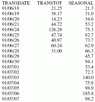
In the following, the data has seasonality but no trend. Therefore, npoint2 is set high (1000) to make the trend factor negligible in the calculation:
TABLE FILE VIDEOTRK
SUM TRANSTOT
COMPUTE SEASONAL/D10.1 = FORECAST_SEASONAL(MODEL_DATA,TRANSTOT,1,3,3,3,1000,1);
BY TRANSDATE
WHERE TRANSDATE NE '19910617'
ON TABLE SET STYLE *
GRID=OFF,$
ENDSTYLE
END
In the output, npredict is 3. Therefore, three periods (nine points, nperiod * npredict) are generated.
