Overview - Fixed and Random Effects
Experimentation is sometimes mistakenly thought to involve only the manipulation of levels of the independent variables and the observation of subsequent responses on the dependent variables. Independent variables whose levels are determined or set by the experimenter are said to have fixed effects.
There is a second class of effects, however, which is often of great interest to the researcher. Random effects are classification effects where the levels of the effects are assumed to be randomly selected from an infinite population of possible levels. Many independent variables of research interest are not fully amenable to experimental manipulation, but nevertheless can be studied by considering them to have random effects.
For example, the genetic makeup of individual members of a species cannot at present be (fully) experimentally manipulated, yet it is of great interest to the geneticist to assess the genetic contribution to individual variation on outcomes such as health, behavioral characteristics, etc. As another example, a manufacturer might want to estimate the components of variation in the characteristics of a product for a random sample of machines operated by a random sample of operators. The statistical analysis of random effects is accomplished by using the random effects model if all of the independent variables are assumed to have random effects, or by using the mixed model if some of the independent variables are assumed to have random effects and other independent variables are assumed to have fixed effects. The Variance Estimation and Precision module provides a comprehensive set of techniques for analyzing research designs that include random effects.
Properties of Random Effects
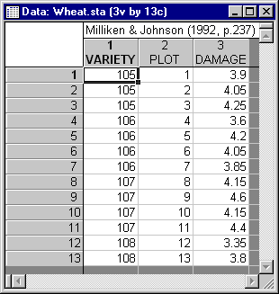
To illustrate some of the properties of random effects, suppose you collected data on the amount of insect damage done to different varieties of wheat. It is impractical to study insect damage for every possible variety of wheat, so to conduct the experiment, you randomly select four varieties of wheat to study. Plant damage is rated for up to a maximum of four plots per variety. Ratings are on a 0 (no damage) to 10 (great damage) scale. The following data for this example are presented in Milliken and Johnson (1992, p. 237); this data set is also provided in the example data file Wheat.sta.
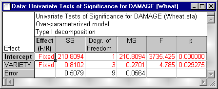
To determine the components of variation in resistance to insect damage for Variety and Plot, an ANOVA can first be performed. Perhaps surprisingly, in the ANOVA, Variety can be treated as a fixed or as a random factor without influencing the results (provided that the Type I option button on the Define/Review Model dialog is selected and that Variety is always entered first in the model). The spreadsheet below shows the ANOVA results of a mixed model analysis treating Variety as a fixed effect and ignoring Plot, (treating the plot-to-plot variation as a measure of random error).
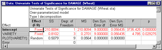
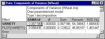
Another way to perform the same mixed model analysis is to treat Variety as a fixed effect and Plot as a random effect. The spreadsheet below shows the ANOVA results for this mixed model analysis.
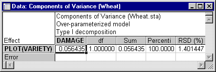
The spreadsheet below shows the ANOVA results for a random effect model treating Plot as a random effect nested within Variety, which is also treated as a random effect.
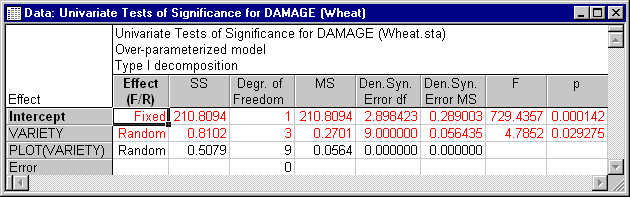
As can be seen, the tests of significance for the Variety effect are identical in all three analyses (and in fact, there are even more ways to produce the same result). When components of variance are estimated, however, the difference between the mixed model (treating Variety as fixed) and the random model (treating Variety as random) becomes apparent. The spreadsheet below shows the variance component estimates for the mixed model treating Variety as a fixed effect.
The spreadsheet below shows the variance component estimates for the random effects model treating Variety and Plot as random effects.
As can be seen, the difference in the two sets of estimates is that a variance component is estimated for Variety only when it is considered to be a random effect. This reflects the basic distinction between fixed and random effects. The variation in the levels of random factors is assumed to be representative of the variation of the whole population of possible levels. Thus, variation in the levels of a random factor can be used to estimate the population variation. Even more importantly, covariation between the levels of a random factor and responses on a dependent variable can be used to estimate the population component of variance in the dependent variable attributable to the random factor. The variation in the levels of fixed factors is instead considered to be arbitrarily determined by the experimenter (the experimenter can make the levels of a fixed factor vary as little or as much as desired). Thus, the variation of a fixed factor cannot be used to estimate its population variance, nor can the population covariance with the dependent variable be meaningfully estimated. With this basic distinction between fixed effects and random effects in mind, we now can look more closely at the properties of variance components.