General Classification and Regression Trees Introductory Overview
Overview
Basic Ideas
The Stastica General Classification and Regression Trees module (GC&RT) will build classification and regression trees for predicting continuous dependent variables (regression) and categorical predictor variables (classification). The program supports the classic C & RT algorithm popularized by Breiman et al. (Breiman, Friedman, Olshen, & Stone, 1984; see also Ripley, 1996), and includes various methods for pruning and cross-validation, as well as the powerful v-fold cross-validation methods. In addition, with this program you can specify ANCOVA-like experimental designs (see MANOVA and GLM) with continuous and categorical factor effects and interactions, i.e., to base the computations on design matrices for the predictor variables. A general introduction to tree-classifiers, specifically to the QUEST (Quick, Unbiased, Efficient Statistical Trees) algorithm, is also presented in the context of the Classification Trees Analysis facilities, and much of the following discussion presents the same information, in only a slightly different context. Another, similar type of tree building algorithm is CHAID (Chi-square Automatic Interaction Detector; see Kass, 1980); a full implementation of this algorithm is available in the General CHAID Models module of Stastica.
Classification and Regression Problems
Stastica contains numerous algorithms for predicting continuous variables or categorical variables from a set of continuous predictors and/or categorical factor effects. For example, in GLM (General Linear Models) and GRM (General Regression Models), you can specify a linear combination (design) of continuous predictors and categorical factor effects (e.g., with two-way and three-way interaction effects) to predict a continuous dependent variable. In GDA (General Discriminant Function Analysis), you can specify such designs for predicting categorical variables, i.e., to solve classification problems.
Regression-type problems. Regression-type problems are generally those where one attempts to predict the values of a continuous variable from one or more continuous and/or categorical predictor variables. For example, you may want to predict the selling prices of single family homes (a continuous dependent variable) from various other continuous predictors (e.g., square footage) as well as categorical predictors (e.g., style of home, such as ranch, two-story, etc.; zip code or telephone area code where the property is located, etc.; note that this latter variable would be categorical in nature, even though it would contain numeric values or codes). If you used simple multiple regression, or some general linear model (GLM) to predict the selling prices of single family homes, you would determine a linear equation for these variables that can be used to compute predicted selling prices. STATISTICA contains many different analytic procedures for fitting linear models (GLM, GRM, Regression), various types of nonlinear models (e.g., Generalized Linear/Nonlinear Models (GLZ), Generalized Additive Models (GAM), etc.), or completely custom-defined nonlinear models (see Nonlinear Estimation), where you can type in an arbitrary equation containing parameters to be estimated by the program. The General CHAID Models (GCHAID) module of STATISTICA also analyzes regression-type problems, and produces results that are similar (in nature) to those computed by GC&RT. Note that various neural network architectures [available in Statstica Automated Neural Networks (SANN)] are also applicable to solve regression-type problems.
Classification-type problems. Classification-type problems are generally those where one attempts to predict values of a categorical dependent variable (class, group membership, etc.) from one or more continuous and/or categorical predictor variables. For example, you may be interested in predicting who will or will not graduate from college, or who will or will not renew a subscription. These would be examples of simple binary classification problems, where the categorical dependent variable can only assume two distinct and mutually exclusive values. In other cases one might be interested in predicting which one of multiple different alternative consumer products (e.g., makes of cars) a person decides to purchase, or which type of failure occurs with different types of engines. In those cases there are multiple categories or classes for the categorical dependent variable. Stastica contains a number of methods for analyzing classification-type problems and to compute predicted classifications, either from simple continuous predictors (e.g., binomial or multinomial logit regression in GLZ), from categorical predictors (e.g., Log-Linear analysis of multi-way frequency tables), or both (e.g., via ANCOVA-like designs in GLZ or GDA). The General CHAID Models module of STATISTICA also analyzes classification-type problems, and produces results that are similar (in nature) to those computed by GC&RT. Note that various neural network architectures [available in STATISTICA Automated Neural Networks (SANN)] are also applicable to solve classification-type problems.
Classification and Regression Trees (C&RT)
In most general terms, the purpose of the analyses via tree-building algorithms is to determine a set of if-then logical (split) conditions that permit accurate prediction or classification of cases.
Classification Trees
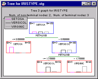
The interpretation of this tree is straightforward: If the petal width is less than or equal to 0.8, the respective flower would be classified as Setosa; if the petal width is greater than 0.8 and less than or equal to 1.75, then the respective flower would be classified as Versicol; else, it belongs to class Virginic.
Regression Trees
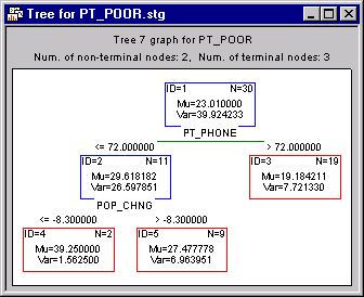
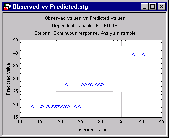
Again, the interpretation of these results is rather straightforward: Counties where the percent of households with a phone is greater than 72% have generally a lower poverty rate. The greatest poverty rate is evident in those counties that show less than (or equal to) 72% of households with a phone, and where the population change (from the 1960 census to the 1970 census) is less than -8.3 (minus 8.3). These results are straightforward, easily presented, and intuitively clear as well: There are some affluent counties (where most households have a telephone), and those generally have little poverty. Then there are counties that are generally less affluent, and among those the ones that shrunk most showed the greatest poverty rate.
A quick review of the scatterplot of observed vs. predicted values shows how the discrimination between the latter two groups is particularly well "explained" by the tree model.