Linear Regression (HD)
Use the Linear Regression operator to fit a trend line to an observed data set, in which one of the data values - the dependent variable - is linearly dependent on the value of the other causal data values or variables - the independent variables.

Information at a Glance
|
Parameter |
Description |
|---|---|
| Category | Model |
| Data source type | HD |
| Send output to other operators | Yes |
| Data processing tool | MapReduce, Spark |
For more information about using linear regression, see Fitting a Trend Line for Linearly Dependent Data Values.
Algorithm
The TIBCO Data Science – Team Studio Linear Regression operator applies a Multivariate Linear Regression (MLR) algorithm to the input data set. For MLR, a Regularization Penalty Parameter that can be applied in order to prevent the chances of over-fitting the model.
This Linear Regression operator implements either Ordinary or Elastic Net Linear Regression.
The Ordinary Regression algorithm uses the Ordinary Least Squares (OLS) method of regression analysis, meaning that the model is fit such that the sum-of-squares of differences of observed and predicted values is minimized.
The Elastic Net Regression algorithm supports the Ordinary Least Squares (OLS) method of linear regression, along with implementing the Elastic Net Objective Function to support either Lasso(L1) or Ridge (L2) penalty cost functions.
This Linear Regression operator implements Ordinary Linear Regression with an option for the Elastic Net Regularization feature to avoid over-fitting a model with too many variables.
Input
A data set that contains the dependent and independent variables for modeling.
Configuration
| Parameter | Description |
|---|---|
| Notes | Notes or helpful information about this operator's parameter settings. When you enter content in the Notes field, a yellow asterisk appears on the operator. |
| Dependent Column | The dependent column specified for the regression. This is the quantity to model or predict. The list of the available data columns for the Regression operator are displayed. Select the data column to consider the dependent variable for the regression.
The Dependent Column should be a numerical data type. |
| Maximum Number of Iterations | The total number of iterations that are processed before the algorithm stops, if the coefficients do not converge or show relevance.
Default value: 20. |
| Tolerance | Maximum allowed error value for the calculation method. When the error is smaller than this value, the linear regression model training stops.
Default value: 0.000001. |
| Columns | Click
Select Columns to select the available columns from the input data set for analysis.
For a linear regression, select the independent variable data columns for the regression analysis or model training. You must select at least one column or one interaction variable. |
| Interaction Parameters | Enables selecting available independent variables, where those data parameters might have a combined effect on the dependent variable. See Interaction Parameters dialog for detailed information. |
| Number of Cross Validation | Gives an option for either 5 or 10 cross-validation steps for the linear regression.
This parameter applies only if Type of Linear Regression is set to Elastic Net Penalty. Cross validation is a technique for testing the model during the training phase by using a small amount of the data as "test" data. Cross validation helps avoid over-fitting a model and provides insight on how the model generalizes to an independent data set. The Number of Cross Validation steps specifies how many times to section off the data for testing. The higher the number of steps, the more accurate the calculated model error is (although the model processing time is greater). Default value: 5. |
| Type of Linear Regression | Determines whether to perform an
Ordinary linear regression or a linear regression with
Elastic Net Penalty applied.
|
| Use Intercept? | Provides the option to calculate the Intercept value,
 , for the linear regression. , for the linear regression.
This parameter applies only if Type of Linear Regression is set to Elastic Net Penalty. In general, this should always be used unless the data has already been normalized. Default value: Yes. |
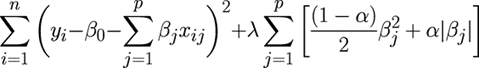
| Penalizing Parameter (λ) | Represents an optimization parameter for linear regression. It implements regularization of the trade-off between model bias (significance of loss function) and the regularization portion of the minimization function (variance of the regression correlation coefficients).
The value can be any number 0 or greater, with the default value of 0 (for no penalty). The higher the Lambda, the lower chance of over-fitting with too many redundant variables. Over-fitting is the situation where the model does a good job "learning" or converges to a low error for the training data but does not do as well for new, non-training data. In general, use regularization to avoid overfitting, so multiple models with different lambda should be trained, and the model with the smallest testing error should be chosen. The lambda value should be greater than 0. For linear regression equations, you can use the cross-validation process to pick the best Lambda value. If you choose a cross validation number, Penalizing Parameter is disabled. The number of cross validations in the results suggest the initial value of lambda. For more information, see Fitting a Trend Line for Linearly Dependent Data Values. |
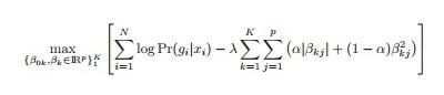
| Elastic Parameter (α) | A constant value between 0 and 1 that controls the degree of the mix between L1 (Lasso) and L2 (Ridge) regularization. Specifically, it is the α parameter in the Elastic Net Regularization loss function given by:
The Elastic Parameter combines the effects of both the Ridge and Lasso penalty constraints. Both types of penalties shrink the values of the correlation coefficients. This parameter applies only if Type of Linear Regression is set to Elastic Net Penalty.
|
| Use Spark | If Yes (the default), uses Spark to optimize calculation time. |
| Advanced Spark Settings Automatic Optimization |
|
Output
Because data scientists expect model prediction errors to be unstructured and normally distributed, the Residual Plot and Q-Q Plot together are important linear regression diagnostic tools, in conjunction with R2, Coefficient and P-value summary statistics.
The remaining visual output consists of Summary, Data, Residual Plot, and Q-Q Plot.
An additional output Cross Validation Plot tab is displayed when an Elastic Net Penalty linear regression is implemented.
- Summary
- Data
- Residual Plot (optional)
- Q-Q Plot (optional)
- Cross Validation Plot
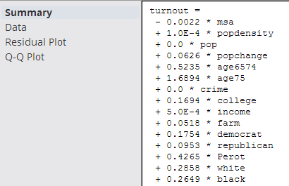
The derived linear regression model is shown as a mathematical equation linking the Dependent Variable (Y) to the independent variables (X1, X2, etc.). It includes the scaling or Coefficient values (β1, β2, etc.) associated with each independent variable in the model.
The following overall model statistical fit numbers are displayed.
- R2: it is called the multiple correlation coefficient of the model, or the Coefficient of Multiple Determination. It represents the fraction of the total Dependent Variable (Y) variance explained by the regression analysis, with 0 meaning 0% explanation of Y variance and 1 meaning 100% accurate fit or prediction capability.
Note: in general, an R2 value greater than .8 is considered a good model. However, this value is relative and in some situations just getting an improved R2 from .5 to .6, for example, would be beneficial.
- S: represents the standard error per model (often also denoted by SE). It is a measure of the average amount that the regression model equation over-predicts or under-predicts.
The rule of thumb data scientists use is that 60% of the model predictions are within +/- 1 SE and 90% are within +/- 2 SEs.
For example, if a linear regression model predicts the quality of the wine on a scale between 1 and 10 and the SE is .6 per model prediction, a prediction of Quality=8 means the true value is 90% likely to be within 2*.6 of the predicted 8 value (that is, the real Quality value is likely between 6.8 and 9.2).
In summary, the higher the R2 and the lower the SE, the more accurate the linear regression model predictions are likely to be.
| Column | Description |
|---|---|
| Coefficient | The model coefficient, β, indicates the strength of the effect of the associated independent variable on the dependent variable.
Note: when implementing Elastic Net Regularization, only the Coefficient results are displayed.
In the case where L1 Regularization is applied (α > 0), if the resulting coefficient value is 0 it typically means that this variable is much less relevant to the model (assuming that normalization of the variables was performed beforehand). |
| SE | Standard Error, or SE, represents the standard deviation of the estimated coefficient values from the actual coefficient values for the set of variables in the regression.
It is best practice to commonly expect + or - 2 standard errors, meaning the actual coefficient value should be within 2 SEs of the estimate. Therefore, a modeler looks for the SE values to be much smaller than the associated forecasted coefficient values. Note: SE is not displayed if Elastic Net Regularization is implemented.
|
| T-statistic | The T-statistic is computed by dividing the estimated value of the β Coefficient by its Standard Error, as follows: T= β/SE. It provides a scale for how big of an error the estimated coefficient has.
Note: T-statistic is not displayed if Elastic Net Regularization is implemented.
|
| P-value | The P-value represents the probability of still observing the dependent variable's value if the coefficient value for the independent variable is zero (that is, if p-value is high, the associated variable is not considered relevant as a correlated, independent variable in the model).
Note: A P-value of less than 0.05 is often conceptualized as there being over 95% certainty that the coefficient is relevant.
The P-value is not displayed if Elastic Net Regularization is implemented. The smaller the P-value, the more meaningful the coefficient or the more certainty over the significance of the independent variable in the linear regression model. In summary, when assessing the Data tab results of the Linear Regression operator, a modeler mostly cares about the coefficient values, which indicate the strength of the effect of the independent variables on the dependent variable, and the associated P-values, which indicate how much not to trust the estimated correlation measurement. |
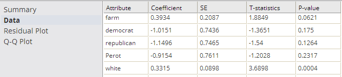
The Residual Plot displays a graph that shows the residuals (differences between the observed values of the dependent variable and the predicted values) of a linear regression model on the vertical axis and the independent variable on the horizontal axis, as shown in the following example.
A modeler should always look at the Residual Plot as it can quickly detect any systematic errors with the model that are not necessarily uncovered by the summary model statistics. It is expected that the Residuals of the dependent variable vary randomly above and below the horizontal access for any value of the independent variable.
If the points in a residual plot are randomly dispersed around the horizontal axis, a linear regression model is appropriate for the data; otherwise, a non-linear model is more appropriate.
A "bad" Residual Plot has some sort of structural bend or anomaly that cannot be explained away.
For example, when analyzing medical data results, the linear regression model might show a good fit for male data but have a systematic error for female data. Glancing at a Residual Plot could quickly catch this structural weakness with the model.
In summary, the Residual Plot is an important diagnostic tool for analyzing linear regression results, allowing the modeler to keep a hand in the data while still analyzing overall model fit.
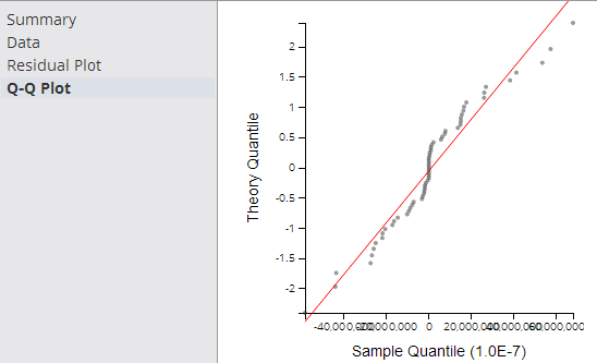
The closer the dots are to the line, the more normal of a distribution the data has. This provides a better sense of whether a linear regression model is a good fit for the data. Any sort of variance from the line for a certain quantile, or section, of data should be investigated and understood.
The Q-Q Plot is an interesting analysis tool, although not always easy to read or interpret.
This graph is only shown when Elastic Net Linear Regression is implemented.
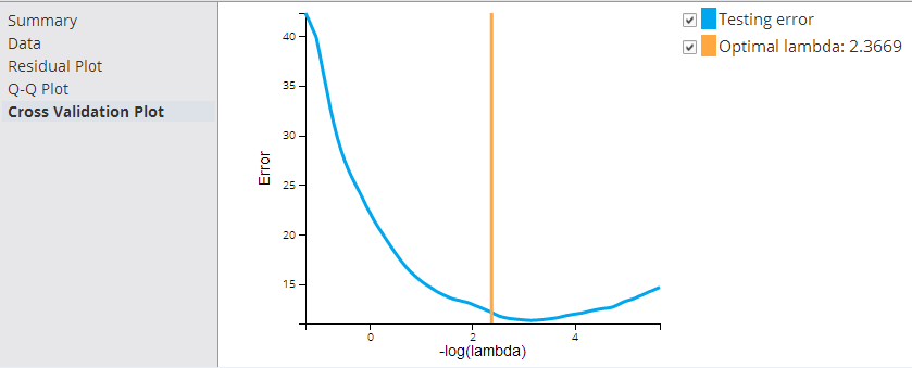
Cross-validation is primarily a way of measuring the predictive performance of a statistical model.
- The best lambda is chosen automatically by the cross validation process. In the example above, the optimal lambda value is 2.3669.
- Lambda controls the degree of regularization with 0 meaning no regularization and infinity meaning ignoring all input variables because all correlation coefficients are turned to zero.
The higher the lambda, λ, the more constraints are imposed on the loss function, as shown in the following formula.
References
- Definition taken from http://www.dtreg.com/linreg.htm
- In actuality, the P-value is derived from the distribution curve of the T-statistic - it is the area under the curve outside of + or - 2*SEs from the estimated Coefficient value.