There are several different models available for curve fitting. See Lines and Curves for information about how to apply the various curves.
Straight Line
The straight line fit is calculated by choosing the line that minimizes the least square sum of the vertical distance d, of all the selected markers (see picture below) by using the following equation:
![]()
where a is the intercept and b is the slope.
For example, you could plot days along the X-axis and have one marker for each day. The distance between the markers along the X-axis is the same, thus making straight line fit appropriate.

Logarithmic
The logarithmic fit calculates the least squares fit through points by using the following equation:
![]()
where a and b are constants and ln is the natural logarithm function. This model requires that x>0 for all data points. Spotfire uses a nonlinear regression method for this calculation. This will result in better accuracy of the calculation compared to using linear regression on transformed values only.
Exponential
The exponential fit calculates the least squares fit through points by using the following equation:
![]()
where a and b are constants, and e is the base of the natural logarithm.
Exponential models are commonly used in biological applications, for example, for exponential growth of bacteria. Spotfire uses a nonlinear regression method for this calculation. This will result in better accuracy of the calculation compared to using linear regression on transformed values only.
Power
The Power fit calculates the least squares fit through points by using the following equation:
![]()
where a and b are constants. This model requires that x>0 for all data points, and either that all y>0 or all y<0. Spotfire uses a nonlinear regression method for this calculation. This will result in better accuracy of the calculation compared to using linear regression on transformed values only.
Logistic Regression
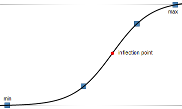
The logistic regression fit is a dose response ("IC50") model, also known as sigmoidal dose response. The four parameter logistic model is the most important one.
Dose-response curves describe the relationship between response to drug treatment and drug dose or concentration. These types of curves are often semi-logarithmic, with log (drug concentration) on the X-axis. On the Y-axis one can show measurements of enzyme activity, accumulation of an intracellular second messenger or measurements of heart rate or muscle contraction.
Note: The logistic regression model of Spotfire is implemented with a setting where you can select whether or not to assume that X is log10-transformed. The default setting is a selected check box, which means that if your input data is not logarithmic, you should make sure to clear the check box in the Edit Curve dialog. You might also want to select the Log scale check box on the X-axis page in the Visualization Properties dialog, to show the values on a logarithmic scale.
Log10-transformed X-values:
The logistic regression on logged X-values fit uses the following equation:
![]()
The LoggedX50 value is interpreted as the Log10(X50). For example, if the H30+ concentration at IC50 has a pH of 3, then the LoggedX50 = -3.
Note: With this model, it is the logged X50 values that are estimated and not the actual X50.
Non-logarithmic X-values:
The logistic regression fit when not assuming logged X-values uses the following equation:
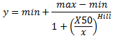
where min and max are the lower and upper asymptotes of the curve, Hill is the slope of the curve at its midpoint and X50 is the x-coordinate of the inflection point (x, y). This model requires that x>0 for all data points and that you use at least four records to calculate the curve.
Polynomial
The polynomial curve fit calculates the least squares fit through points by using the following equation:
![]()
where a0, a1, a2, etc., are constants. The default order is a 2nd order polynomial, but you can change the degree in the Edit Curve dialog. This model requires that you use at least three markers to calculate the curve for a 2nd order polynomial model, and four markers for a 3rd order polynomial, etc.
If you have a low number of unique x-values, a polynomial curve can be calculated in an unlimited number of ways. This means that you may end up with a curve that does not look as expected. If this should happen, you probably should not apply this model to your data.
Some of the models have been partially solved by using the LAPACK software package, see References.
Gaussian
The Gaussian curve fit calculates a bell curve suitable to describe normal distributions using the following equation:
![]()
where A is the amplitude of the curve, E is the position of the center of the curve and G is the width.
In TIBCO Spotfire, you have the possibility to let the application calculate values on the parameters A, E and G automatically from the available data. You can also specify one or more of the parameters yourself.
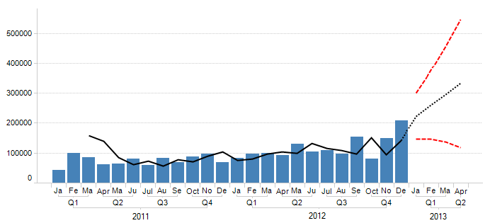
The Holt-Winters Forecast uses TIBCO Spotfire Enterprise Runtime for R to compute the Holt-Winters filtering of a time series or anything that can be coerced to a time series. This is an exponentially weighted moving average filter of the level, trend, and seasonal components of a time series. The smoothing parameters are chosen to minimize the sum of the squared one-step ahead prediction errors.
The output of a Holt-Winters Forecast is three different curves: a fitted curve showing the general variation of the measure of interest, a forecast curve predicting the future trend and a confidence interval showing how the insecurity increases the further away from the known values the prediction reaches.
TIBCO Enterprise Runtime for R and open-source R return different prediction intervals for multiplicative seasonal models. TIBCO Enterprise Runtime for R assumes that the seasonal and error components are multiplicative in effect and it uses the formula for prediction variance found in section 6.4.2 of Hyndman, et al, 2008. See the references listed in the References section.
The used parameters can be shown in labels or tooltips.
See also: