A pivot transformation is one way to transform data from a tall/skinny format to a short/wide format. The data is distributed into columns usually aggregating the values. This means that multiple values from the original data end up in the same place in the new data table.
Example:
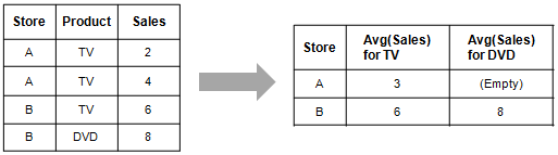
The example below shows a pivot transformation on a very simple data set. In the original data table, there are three columns and four rows. Each row contains one of two department stores, A or B; a product, TV or DVD; and a numerical value for the number of sales. The data table might look like this if a new row is added after each day.
However, perhaps we are more interested in knowing how many units of each product are sold in each store on an average day.
After pivoting the data table, using the aggregation method "average" on the numerical values for the two products, we get a new data table. This data table has just two rows, one for each store. The layout of the table has gone from tall/skinny to short/wide. Had there been more products in the data table the difference would be even more pronounced. In the new data table, it is easy to see the number of products being sold in each store on an average day. The first row tells us that on any given day in department store A, 3 TVs are sold, but no DVDs. In department store B, however, an average day might see 6 TVs and 8 DVDs sold.
Example:
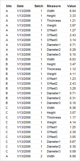
In this example, we have a larger data set, with data from an imagined company that produces small machinery parts. These parts have measurements for width, height and thickness. The parts have three different holes in them. There are also measurements for the diameter of these holes, and a measurement for a possible small offset from where they are supposed to be.
In the original data table, which contains measurements for samples of all parts, we can see which of the company's three factories—A, B or C—have produced the parts, and we can see on which date the parts were shipped, which batch they belong to as well as all the measurements for the parts.
What we are really interested in knowing is how good the three different factories are at producing these parts. If we deliver the parts to different customers who have different demands for the accuracy of the holes in the part, we want to know which factory should supply which customer with parts. We then pivot the data to get one row for each factory, and to get minimum, maximum and average values for the different measurements of the parts.
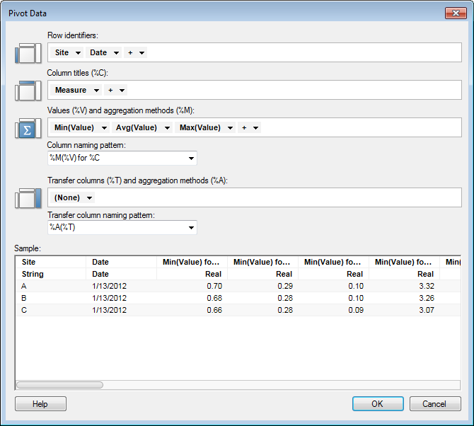
The order of the new columns is determined by the result of the naming expression, sorted in alphabetic order.
After importing the data to Spotfire, we can start analyzing it. By filtering the data, we can set the minimum and maximum allowed measurements for the diameter and offset of the holes in the part.
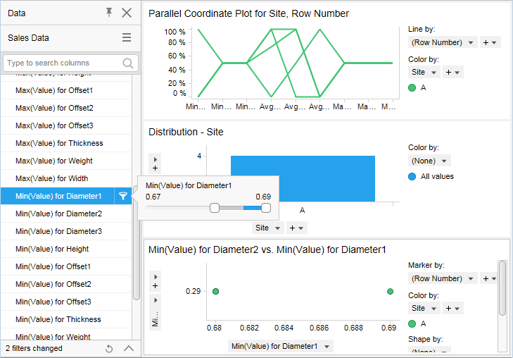
In the analysis, we can see that if the most important criterion is that the diameter is not too small, A is the factory that should supply parts to the most demanding customers.
See also: