Example 4: Weibull and Reliability/Failure Time Analysis
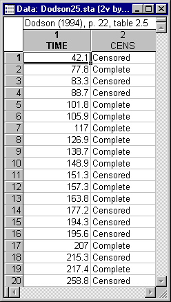
This example is based on a data set presented in Dodson (1994, Table 2.5). No specific information is provided regarding the origin of these data, however, the data set is an example of multiple-censored failure time data. The example data are available in the example data file Dodson25.sta. Open this data file via the File - Open Examples menu; it is in the Datasets folder.
The goal of the analysis is to fit the Weibull distribution to these data, and to estimate the percentiles of the reliability function.
- Specifying the Analysis
- Select Process Analysis from the Statistics -
Industrial Statistics & Six Sigma submenu to display the Process Analysis Procedures Startup Panel. Here, double-click
Weibull analysis & reliability/failure time analysis to display the
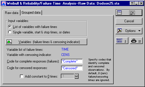
Weibull & Reliability/Failure Time Analysis dialog box.
On the Raw data tab, click the Variables (failure times & censoring indicator) button to display a standard variable selection dialog box. Select variable Time as the variable with Failure times, variable Cens as the Censoring indicator variable, and then click the OK button.
Now, double-click the Code for complete responses (failures) field to display the Variable 2 dialog box. Select Complete and then click the OK button. In the same manner, select Censored as the Code for censored responses.
Then click the OK button to start the analysis.
- Default Fit
- After reading the data, Statistica will by default compute maximum likelihood parameters for the two-parameter Weibull distribution, assuming the location parameter to be equal to zero. The Weibull Analysis Results - Quick tab will show these estimates in the Current parameter values/estimates box.
- Estimating parameters
- The Advanced tab contains options to explore interactively the fit of the Weibull distribution with different parameters. When you select the ML shape & scale parameters option button, the Recompute button becomes available. When you click the Recompute button, Statistica will "read" the current value of the Offset (threshold/location) parameter, and then compute maximum likelihood parameter estimates for the Shape and Scale parameters based on the respective Offset (threshold/location) parameter. If you select the ML location, shape, scale parameters option button, Statistica will compute maximum likelihood parameter estimates for the three-parameter Weibull distribution. In either case, the resulting parameter estimates are displayed as the Parameter values/estimates, in the respective edit fields.
- Reviewing results
- All options available on the Results dialog will compute spreadsheets and graphs based on the current set of parameters, as specified in the Parameter values/estimates box, regardless of whether or not the current parameter values were estimated (i.e., maximum likelihood estimates) or otherwise specified by the user. (However, standard errors for the reliability function can only be computed for maximum likelihood parameter estimates).
- Estimates based on probability plotting
- The maximum likelihood estimates for the two-parameter Weibull distribution are 2.97 and 203.3 for the
Shape and
Scale parameter, respectively. You can compare these against the estimates derived from probability plotting: First on the
Reliability & distribution function tab, select the
Nonparametric option button under Conf. intervals. This will cause all plots to be based on a nonparametric (rank-based) estimate of the cumulative distribution function F(t), and the resulting probability plots can be used to estimate the parameters for the Weibull distribution (see also the
Introductory Overview). Click the
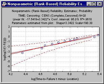
Probability plot button to produce the graph.
This plot shows the observed failure data, the linear fit line (in blue), the 95% nonparametric confidence interval for the reliability (i.e., the log-log transformation, as indicated by the y-axis label in the plot shown above; the confidence interval is indicated by the red dotted lines), and the center (50th percentile) of the nonparametric confidence interval (indicated by the dashed red line). As briefly described in the Introductory Overview, you can estimate the shape and scale parameters from the slope and intercept of the linear fit line in this plot; specifically, the shape parameter is equal to the slope of the linear fit-line, and the scale parameter can be estimated as exp(-intercept/slope). The resultant estimates for this specific plot, 3.34 and 190.3 for the Shape and Scale parameters, respectively, are very similar to the maximum likelihood parameter estimates. Also, because the points in this plot are well represented by the fitted line (R2 is equal to .96), we have reason to believe that the Weibull distribution with these parameters provides an adequate fit to the data.
- Goodness of fit tests
- If you click the
Goodness of fit tests button on the
Advanced tab, you will see that neither the
Hollander-Proschan nor the
Mann-Scheuer-Fertig test statistic is significant, further indicating a satisfactory fit to the data.
Refer to the Introductory Overview for additional details about these tests.
- Estimating a location parameter
- Even though the fit for the two-parameter Weibull distribution appears to be very good, suppose we have reason to believe that the true location parameter is greater than zero, i.e., that there is a certain amount of time (greater than zero) during which the probability of failure is equal to zero. Let us therefore estimate a location parameter. First click the R2 vs. location parameter button on the
Advanced tab. This graph shows the resultant R2 value for the probability plot produced based on the location parameter values scaled along the x-axis.
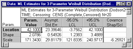
It is apparent from this plot that the R2 value steadily increases up to a value very close to the smallest (censored) failure time recorded in the data. (In other cases, you may see a curve with a single peak; see, for example, Figure 2.6 in Dodson, 1994.) Next, on the Advanced tab, select the ML location, shape, scale parameters option button to compute the maximum likelihood estimates for the three-parameter Weibull distribution; then click the Summary: Parameters button to review the parameters and their standard errors.
Evidently, even though the Location parameter is estimated as 42.1, the 95% confidence limits include 0, and therefore, we will accept the (simpler) two-parameter model, with the location parameter equal to zero. Select the ML shape & scale parameters option button and then enter 0 in the Offset (threshold/location) box. Next, click the Recompute button and then click the Summary: Parameters button again to compute the maximum likelihood parameter estimates for the two-parameter distribution.
- Percentiles and confidence limits
- Next click the
Percentiles and confidence limits button on the
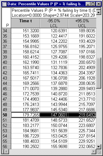
Reliability & distribution function tab to display the spreadsheet with the percentile values for the reliability function.
The spreadsheet shows the percentile values in one percent increments, i.e., for percentile 1, 2, 3, 4, and so on. For example, for the 50th percentile, the time value is equal to 179.73, with a 95% confidence interval from 147.06 to 219.65. In other words, 50% of all items can be expected to have failed prior to t=179.73 (with the respective confidence interval).
- A note of caution regarding maximum likelihood based confidence limits
- Dodson (1994) cautions against the reliance on confidence limits computed from maximum likelihood estimates, or more precisely, estimates that involve the information matrix for the estimated parameters. When the shape parameter is less than 2, the variance estimates computed for maximum likelihood estimates lack accuracy, and it is advisable to compute the various results graphs based on nonparametric confidence limits as well.

