Example 2: Log Linear Analysis of Frequency Tables (incomplete)
This example is based on a classic data set reported by Morrison, et al. (1973) and discussed by Bishop, Fienberg, and Holland (1975).
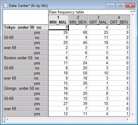
The data is contained in the data file Center.sta that is included with your Statistica program. The data file contains a frequency table of the number of breast cancer patients who survived three years or longer after the diagnosis (obviously, this data is not representative of the chances of surviving breast cancer today).
The frequencies are reported separately for four different types of inflammation and appearance (MIN_MAL, MIN_BEN, GRT_MAL, GRT_BEN), three age groups (under 50, 50-69, over 69), and separately for three diagnostic centers (Tokyo, Boston, and Glamorgan). The complete table was entered into the spreadsheet, which is shown in the following image.
Goal of the analysis
In general, the goal of log-linear analysis of a frequency table is to uncover relationships between the categorical variables (factors) that make up the table. The Introductory Overview introduces the distinction between design variables and response variables, a distinction that basically corresponds to that between independent and dependent variables, respectively. The major response variable of interest in this table is Survival. All other factors are treated as design factors. Thus, you will not be concerned with any interactions between, for example, the location of the diagnostic center and the age of the patients or the appearance of the cancer.