Example 7: Distributed Lags Analysis
Overview and Data File
This example is based on data published by the US Education Department. The file Teachers.sta contains data describing;
- The number of students enrolled in public schools (variable Children),
- The number of public school teachers (Teachers), and
- The average salary of public school teachers (Salary).
These data are presented for the period from 1900 through 1980, in ten-year intervals. Open this data file via the File - Open Examples menu; it is in the Datasets folder.
It is reasonable to assume that the number of teachers employed in the public schools will be a function of the number of students that are in the schools. However, you may expect some lag in the relationship. When, due to demographic changes, there are many students, there will be more hiring of teachers; however, it will take some time to "produce" those teachers. Greater demand for teachers should also drive up the salaries, again, probably with some lag.
Specifying the Analysis
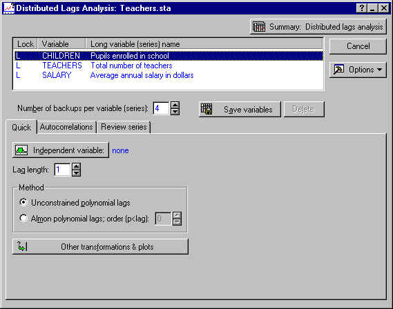
Select Time Series/Forecasting from the Statistics - Advanced Linear/Nonlinear Models menu to display the Time Series Analysis Startup Panel. Click the Variables button to display the standard variable selection dialog. Here, select all variables and click the OK button. Now, click the Distributed lags analysis button to display the Distributed Lags Analysis dialog.
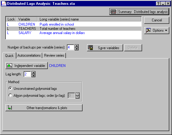
Begin this example by analyzing the number of teachers as the dependent variable; the independent or explanatory variable is the number of school children. To select the dependent variable, highlight Teachers in the active work area; then click the Independent variable button to display the Currently available variables and transformations dialog. Select Children as the independent variable and click the OK button. Next, set the Lag length to 2 to look at a 10-year and 20-year lag.
Reviewing Results
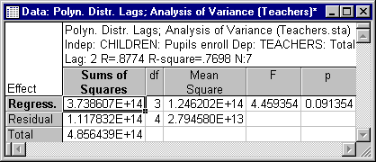
Click the Summary: Distributed lags analysis button to begin the analysis. The results will be displayed in two spreadsheets.
The results show that there is a strong but only marginally significant correlation between variables (R = .88). However, note that the regression computations in distributed lags analysis do not allow for an intercept in the equation (as is apparent in the equation presented in the Introductory Overview). As with many econometric models, the intercept of the regression line is assumed to be zero, since, if there are no students, there would not be any teachers either.
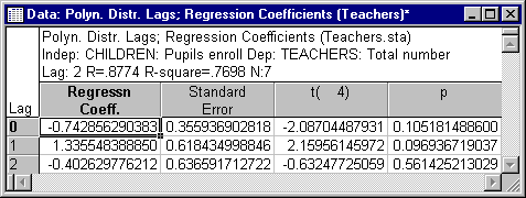
Regression coefficients
Judging from the results shown above, there is indication of a 10-year lagged effect; that is, the t value for Lag = 1 (and for Lag = 0) is greater than 2. Of course, because of the small number of cases in this file, this t value is not statistically significant.
Salary
As before, the largest t value is in the second row of the spreadsheet, denoting the 10-year lag.
Conclusion
The results of these analyses lend some support to the hypothesis that the number of teachers and their salaries "respond" to the number of students with a lag.
Almon Distributed Lag
As described in the Introductory Overview, the standard multiple regression estimates for lags analysis sometimes suffer from multicollinearity problems. Now repeat the analyses using the Almon distributed lags method. On the Distributed Lags Analysis - Quick tab, select the Almon polynomial lags option button. Next, highlight variable Teachers in the active work area.
Specifying polynomial order
As described in the Introductory Overview, this technique approximates the regression weights with a polynomial series of length smaller than the lag length. For this example, set the order (p<lag) field to 1. You are now ready to proceed. Click the Summary: Distributed lags analysis button to review the results.
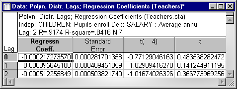
In this case, the t value for the 10-year lag is much larger than that of the other lags, further supporting the hypothesis. If you repeat this analysis for the Salary data (highlight Salary in the active work area and click the Summary: Distributed lags analysis button), you will obtain the following results.
Again, the regression weight for the 10-year lag is the most significant one of the three.
See also, Time Series Analysis Index.


