Example 4: Seasonal and Non-seasonal Exponential Smoothing
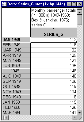
Example 2 discusses the analysis of a data set from the classic book on ARIMA by Box and Jenkins (1976). The data are monthly passenger totals (measured in thousands) in international air travel, for twelve consecutive years: 1949-1960 (see Box and Jenkins, 1976, page 531, "Series G"). The Series_G.sta data file is partially listed below. Open this data file via the File - Open Examples menu; it is in the Datasets folder.
The ARIMA analysis required a good deal of preparatory work during the identification stage. In fact, it usually requires a lot of experience and familiarity not only with ARIMA but also with the nature of the data, in order to identify satisfactory models. Often, the purpose of ARIMA is mostly to derive forecasts, and the interpretation of the nature of the model (i.e., the number and types of parameters) is only of secondary interest. In those cases, exponential smoothing provides a much easier alternative, one that usually produces forecasts of equal or better quality (see the Introductory Overview for a discussion of this point).
In this example, exponential smoothing will be performed on the same series used in Example 2 and the forecasts derived by the two methods will be compared.
Choosing a Model
Even though exponential smoothing is, in a way, a simpler method than ARIMA, some choices still have to be made. Select Time Series/Forecasting from the Statistics - Advanced Linear/Nonlinear Models menu to display the Time Series Analysis Startup Panel. Then, click the Variables button to display the standard variable selection dialog. Here, select the variable Series_G (note that if the data file Series_G.sta is the currently open data file, and since Series_G is the only variable in that data file, then when the Time Series Analysis dialog opens, Series_G will automatically be selected). Click the OK button on the variable selection dialog to return to the Startup Panel. Now, click the Exponential smoothing & forecasting button to proceed to the Seasonal and Non-Seasonal Exponential Smoothing dialog.
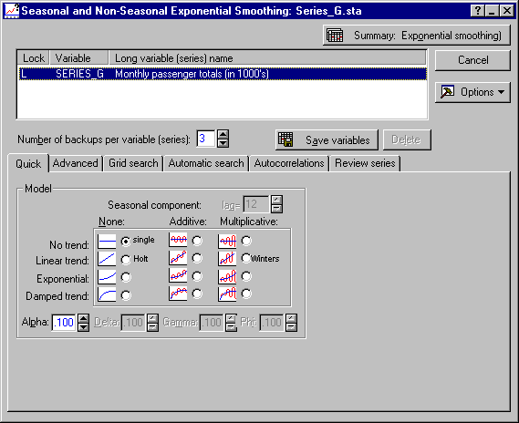
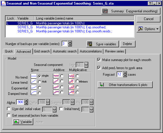
As described in the Introductory Overview, there are different exponential smoothing models available. In general, in all models the smoothed or forecasted values are computed as a weighted average of the preceding values. The difference between the models listed in the Model box is whether or not a trend and/or seasonal component are smoothed with extra smoothing parameters. Examine the differences between models by looking at the results of smoothing with the different techniques and parameters. However, first plot the series. Because Series_G.sta contains dates in the case names, use those to label the horizontal x-axis in line plots. Click on the Review series tab and select the Case names option button. Then select the Scale X axis in plots manually check box and specify Min = 1 and Step = 12 (as there are 12 months in a year). Now, click the Plot button next to the Review highlighted variable button.

The data in this series are easily matched up with the general "model shapes" shown on the icons in the Model box of the Seasonal and Non-Seasonal Exponential Smoothing dialog - Advanced tab. Clearly, there is a trend, which is more or less linear. Second, there is seasonal fluctuation; that is, every year the number of airline passengers follows an almost identical pattern (e.g., most travel occurs during the summer vacation months). This seasonality is multiplicative rather than additive in nature: The higher the overall level of the series the greater is the seasonal fluctuation. Put another way, the increase in airline passenger loads during the summer months each year can best be expressed by a factor; for example, each summer the passenger load increases by a factor of 1.1, or 10%. Thus, the Winters model (Linear trend, Multiplicative) is probably the best exponential smoothing model to use for this series. However, first look at some other models.
Simple Exponential Smoothing
The Forecast box will show 10 cases by default; change this to 12 and forecast one full year. Then, accept all other defaults and click the Summary: Exponential smoothing button. Shown below is the plot of the original and smoothed series, and the residuals.

Two things are immediately apparent. First, the smoothed series traces the general linear trend but fails to follow the seasonal cycles. Second, all forecasts are the same. In fact, if you look back over the description of simple exponential smoothing in the Introductory Overview, this could be expected: Each smoothed value or forecast St is computed as St = St-1 +α * e, where e is the error or observed minus predicted (smoothed or forecasted) value. When there are no observed values available (e.g., when computing forecasts), then e is assumed to be 0 (zero). Thus, all forecasts are the same from then on.
The α (alpha) parameter. Now look at the effect of the smoothing parameter α (alpha). Looking at the formula above, it is clear that as α approaches 0 (zero), all smoothed values will become very similar; when α approaches 1, then the smoothed values should very closely follow the actual observed data. Set the Alpha parameter to .900 on the Advanced tab and select the original Series_G variable in the active work area.
Click the Summary: Exponential smoothing button again.

Now the smoothed values follow the observed values very closely; it almost looks like the original series is simply moved by one observation to the right. Indeed, if you were to set the α (Alpha) parameter to 1, then each smoothed value would be equal to the previous observation. Therefore, in a sense, the α parameter can be considered a stiffness parameter. The smaller the α the "stiffer" the smoothed line; that is, the smoothed line will not be affected as much by the random observation-to-observation variability. The larger the α the more flexible the smoothed line; that is, the more closely will it follow the fluctuations in the observed values. This is generally true for all exponential smoothing models, and this principle applies equally to the seasonality and trend smoothing parameters of the more complex models (see below).
Exponential Smoothing with Linear Trend
Now select Holt Linear trend smoothing (without seasonality). In this model, a trend component is independently smoothed with parameter γ (Gamma). If γ is set to 0, then a constant slope will be included in the computation of smoothed values and forecasts. If γ is set to 1, then the slope is recomputed at each observation from the respective immediately preceding smoothed value; thus, the slope is allowed to change as much as necessary from observation to observation, in order to approximate the observed values. Shown below is the summary plot for two smoothing trials, the first with α = 0.1 and γ = 0.1, the second with α = 0.9 and γ = 0.9. (Be sure to select the original Series_G variable in the active work area before you produce the summary plots.)

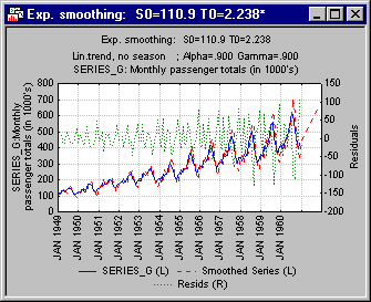
As expected, the smoothed values follow the observed values more closely in the second graph shown above. However, looking at the forecasts it is evident that in this model (without seasonality), the predicted values simply consist of a straight line. Thus, using the Holt two-parameter (Linear trend) model, you would "miss" the significant seasonal increase of airline passengers during the summer months.
Now look at the model that seems most appropriate here, that is, the Winters three-parameter model with Linear trend and Multiplicative seasonality.
Triple Exponential Smoothing: Winters' Method
In this method, a third parameter δ (Delta) is added to the model to smooth the multiplicative seasonal component. Again, if δ is 0 (zero), then a constant stable seasonal component is included in the computation of the smoothed values and forecasts; if δ is set to 1, then the seasonal component is recomputed from observation to observation. Shown below are the summary plots for α = 0.1, δ = 0.1, and γ = 0.1, and for α = 0.9, δ = 0.9, and γ = 0.9.
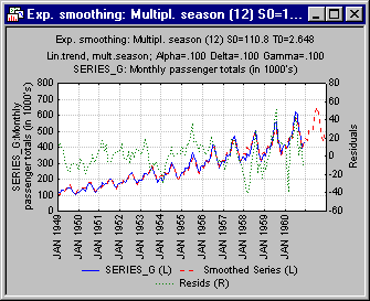
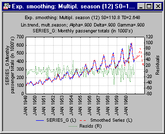
In this case, there is hardly any difference between the two summary plots. The reason for this is that the series indeed consists of a stable linear trend, strong stable seasonal fluctuation, and only little random fluctuation. Therefore, even though by setting δ and γ to 0.9, you "allow" the seasonal and trend components to be modified substantially from observation to observation, no such modification is required. In fact, the automatic search for the best parameters discussed below will arrive at the same conclusion.
Parameter Grid Search
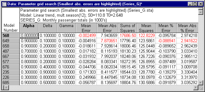
As discussed in the Introductory Overview, in practice, when you want to compute forecasts, you are best advised to estimate optimum smoothing parameters from the data (e.g., see Gardner, 1985). This can be done in two ways. One common method is to perform a grid search of the parameter space. Thus, click on the Grid search tab. STATISTICA will increment each parameter from the minimum (Start parameter at) by the value specified in the Increment by column, up to the value specified in the Stop at column.
For each combination of parameter values, STATISTICA will compute the Sums of Squares (SS) for the residuals (observed values minus smoothed values). By default, when the Display parameters for 10 smallest mean squares check box is selected, then the "best" 10 solutions; that is, the combinations of parameters that yield the smallest residual variability will be displayed in a spreadsheet. Accept all defaults and examine that spreadsheet (see below) by clicking the Perform grid search button. (Be sure to select the original Series_G variable in the active work area before you produce the spreadsheet.) As suspected, the best-fitting models are those with parameter values for δ and γ near 0 (zero), that is, models with constant stable linear trend and seasonality.
Automatic Parameter Search
The second way to determine the optimum parameters for smoothing is to minimize the Sums of Squares of the residuals or some similar index of goodness of fit. This can be done in the Time Series module by using a general nonlinear function minimization algorithm (the so-called quasi-Newton method; the same method used to estimate the ARIMA parameters). Now, click on the Automatic search tab. This tab contains several technical parameters that pertain to the quasi-Newton method; those parameters are described in detail in the Automatic search tab help. The Lack of fit indicator group shows the different quantities that can be minimized.
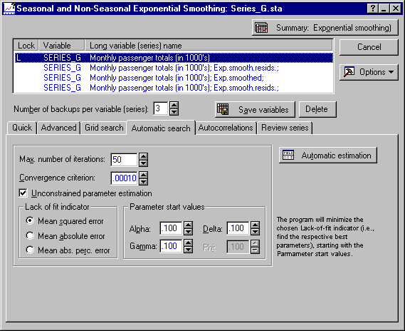
As Parameter start values, specify 0.1 for all three parameters (it is always a good idea to start the minimization procedure with small parameter values). By default, the Unconstrained parameter estimation check box is selected. This means that in the course of the function minimization, you may see parameter values that become smaller than 0 (which is not permissible for the smoothing parameters). However, before the final results are reported, the parameters will automatically be set to the closest valid value, so you do not have to change this setting (again, refer to the description of this option in the Automatic search tab help, for a more detailed discussion). Now click the Automatic estimation button and after the iterative parameter search procedure finishes, look at the summary graph for the best parameter values.
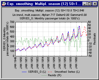
Once again, as in the grid search, the best model is one that contains a stable constant linear trend and seasonality. The remaining random variability is best smoothed with a very "flexible"(large) α parameter value (0.72) that allows the smoothed values to follow closely the observed values.
Final Results
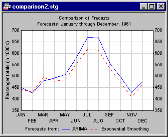
Now return to the original goal, namely to compare the forecasts produced by exponential smoothing with those from ARIMA. Lock the exponentially smoothed values and then compute the ARIMA analysis as described in Example 2. After you complete the ARIMA analysis, go to the Transformations of Variables - Review & plot tab and plot the exponentially smoothed series with the ARIMA forecasts by clicking the Plot two var lists with different scales button.

If you select the Display/plot subset of cases only check box on the Review & plot tab, you can specify to plot the from 1 through 12 forecasts only.
See also, Time Series Analysis Index.