Stepwise Model Builder Example
In this example, the Stepwise Model Builder module is used to create a custom logistic regression model for predicting a credit standing outcome. This analysis tool is the next logical progression from the Weight of Evidence tool. We will use the output from the Weight of Evidence example where the CreditRisk.sta example data set was used to create WoE variables via a Statistica Enterprise analysis configuration. The resulting data spreadsheet, Credit Risk WoE.sta, can be found in the Statistica examples folder.
Starting the analysis. Open the Credit Risk WoE.sta data set, and start the Stepwise Model Builder module:
Ribbon bar. Select the Home tab. In the File group, click the Open arrow and from the menu, select Open Examples. The Open a Statistica Data File dialog box is displayed. Credit Risk WoE.sta is located in the Datasets folder. After opening the data set, select the Statistics tab. In the Advanced/Multivariate group, click Advanced Models and from the menu, select Stepwise Model Builder to display the Stepwise Model Builder Startup Panel.
Classic menus. On the File menu, select Open Examples to display the Open a Statistica Data File dialog box; Credit Risk WoE.sta is located in the Datasets folder. After opening the data set, from the Statistics - Advanced Linear/Nonlinear Models submenu, select Stepwise Model Builder to display the Stepwise Model Builder Startup Panel.
In the Variable Selection group box, click the Select variables button to display the variable selection dialog box. In the Dependent list, select Credit Standing. In the Continuous predictor list, select the variables labeled WoE, variables 16 through 28.
In the Weight of Evidence example, the predictor variables were recoded with weight of evidence values to maximize predictability of the logistic regression model. These recoded variables are used as inputs for this model.
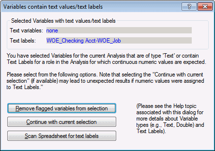
Click the OK button to confirm the selected variables and close the dialog box. A dialog box is displayed that alerts you that a variable contains text labels when continuous data is expected. All the WoE variables use the numeric WoE value and show the grouping as text labels. The variable selection is correct and expected.
Click the Continue with current selection button to continue. The Stepwise Model Builder is updated with the variable selection and the variables are listed in the Marginal Analysis Variables pane.
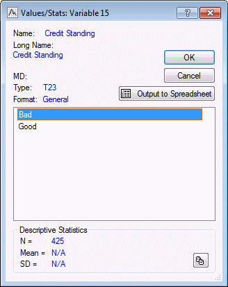
In the Dependent (Y) Variable group box, the Bad code and Good code fields need updated. Double-click in the Bad code field to display the Values/Stats dialog box. Select Bad in the list.
Click OK to update this field and close the dialog box.
Repeat the process to enter Good in the Good code field.
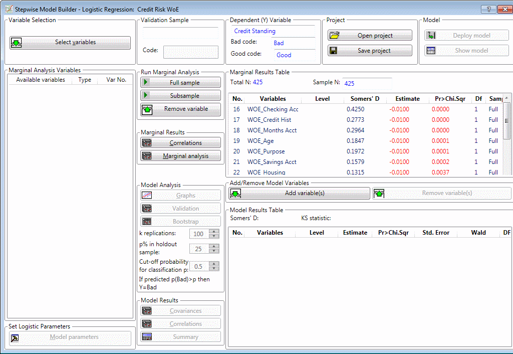
Building the model. In the Run Marginal Analysis group box, click the Full sample button to begin building the logistic regression model. After processing, the Marginal Results Table will be updated with estimates and a p-value for variables in the predictive variable pool.
From experience, it is expected that Checking Account would be an important variable in this model. In the results, this variable, WoE_Checking_Acct, is statistically significant.
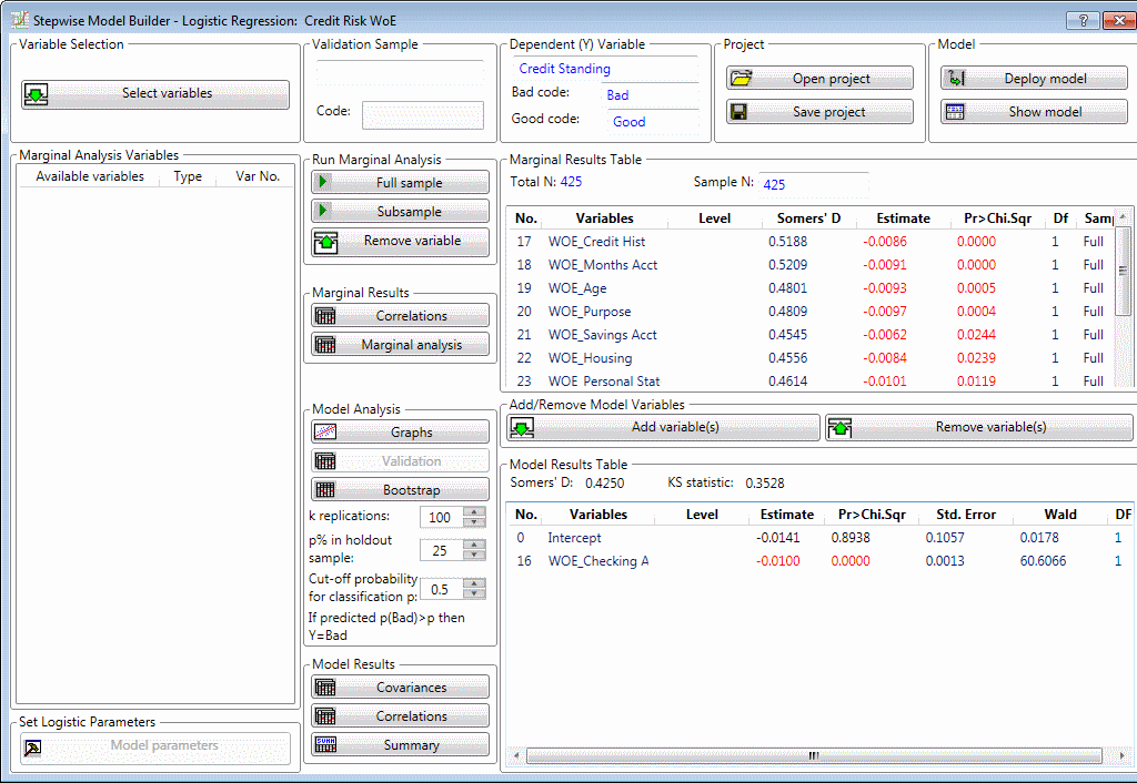
In the Marginal Results Table, select WoE_Checking_Acct. Then, in the Add/Remove Model Variables group box, click the Add variable button.
The Intercept and variable, WoE_Checking_Acct, are added to the model and are displayed in the Model Results Table.
Next, in the Marginal Results group box, click the Marginal analysis button to output a spreadsheet for each remaining variable that can be added to the final model.
Following is the output for the variable WoE_Credit Hist. In this spreadsheet, we see the model parameter estimates and significance tests for the model that include the Intercept and WoE_Checking Acct from the current selected model and the potential variable to add, WoE_Credit Hist. This variable is statistically significant, p=0.000004. It must be considered for the final model.
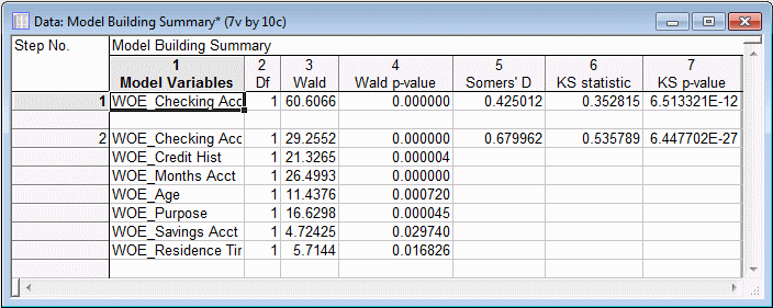
These results can be reviewed for all potential variables to add to the model. Continuing to use a combination of knowledge of the relationships expected in the data and what variables are easiest to track, along with the significance of the available variables, the following variables are also added to the model: Credit History, Months Acct, Age, Purpose, Savings Acct, and Residence Time. The Stepwise Model Builder updates as new variables are added to the final model.
Verifying the model. Once a good model is found containing our selection of variables, we can explore the model. In the Model Analysis group box, click the Graphs button. This creates several pieces of output including the Lift Chart showing the final model’s performance.
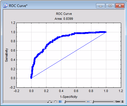
Another graph created in the output is the ROC Curve (Receiver Operating Characteristic Curve). This plot also helps to assess model performance. The greater the area under the curve, the better the model performance.
The model has overall good performance. To get an idea of the distribution of the parameter estimates, we can create bootstrap samples to estimate the distribution of the parameter estimates.
In the Model Analysis group box, confirm that the k replications parameter is set to 100.
Then, click the Bootstrap button to begin the process of taking bootstrap samples with replacement and estimating the model parameters. A message is displayed alerting you that this may take some time; click Yes.
When the process completes, a histogram is plotted for each parameter in the model, and a spreadsheet is created of the model parameter estimates across the 100 bootstrap samples. Following is the histogram of the bootstrap model parameter estimates for the variable WoE_Checking Acct.
Deploying the model. And finally, in the Model Results group box, click the Summary button to output the Model Building Summary and the Parameter estimates.
You can also create an analysis configuration to deploy these results. In the Model box, click the Deploy Model button.


