Example 7: Detecting Outliers

Open the data file:

Ribbon bar. Select the Home tab. In the File group, click the Open arrow and on the menu, select Open Examples. The Open a Statistica Data File dialog box is displayed. Poverty.sta is located in the Datasets folder.

Classic menus. On the File menu, select Open Examples to display the Open a Statistica Data File dialog box; Poverty.sta is located in the Datasets folder.

Ribbon bar. Select the Statistics tab. In the Base group, click Basic Statistics to display the Basic Statistics and Tables Startup Panel.

Classic menus. On the Statistics menu, select Basic Statistics/Tables to display the Basic Statistics and Tables Startup Panel.

To begin the analysis, double-click Descriptive statistics to display the Descriptive Statistics dialog box.

Graphical approach. A common graphical means of detecting outliers is to construct a box plot of the data.

To do this, click the Variables button in the Descriptive Statistics dialog box to display a variable selection dialog box. Because we are interested in detecting any existing outliers, click the Select All button, and then click OK in the variable selection dialog box.

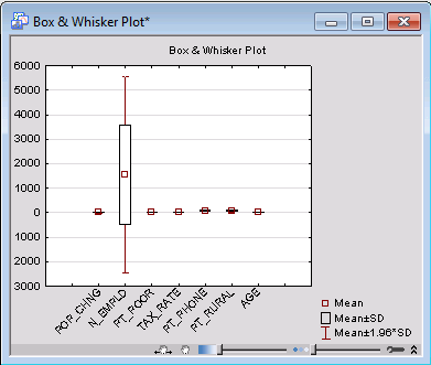
Now, on the Quick tab in the Descriptive Statistics dialog box, click the Box & whisker plot for all variables button.

Clearly, there is greater variability within the variable N_EMPLD than within the other variables.

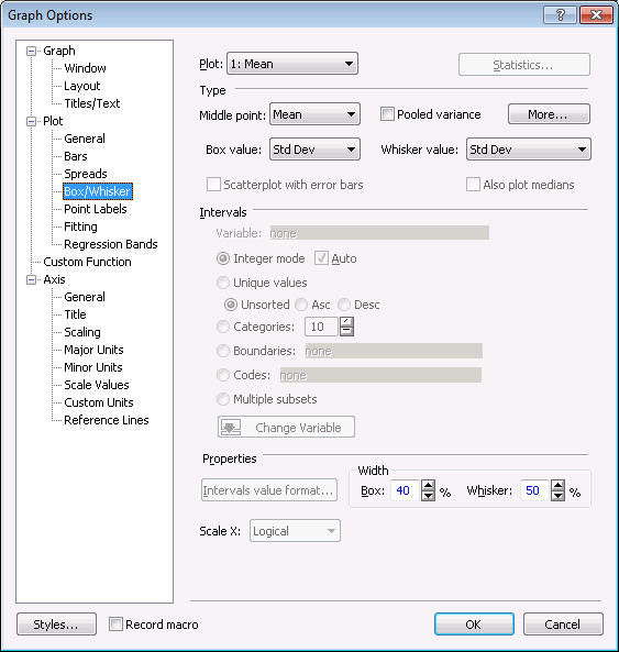
In this initial graph, potential outliers and extreme values are not displayed. To enable this feature, double-click in the background of the graph to display the Graph Options dialog box. Select the Box/Whisker tab (located under Plot).

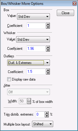
Click the More button to display the Box/Whiskers More Options dialog box, in which you can select additional options to compute the box and whiskers, control the display of outliers and extremes, and use the trimmed distribution of the dependent variable to compute mean/median. In the Outliers drop-down list, select Outl. & Extremes.

Click the Close button in the Box/Whiskers More Options dialog box, and click the OK button in the Graph Options dialog box to update the graph with outliers and extreme values.

As we suspected, there seems to be an outlier in the variable N_EMPLD.

Grubbs test. The Basic Statistics and Tables module also provides certain quantitative methods for detecting outliers, one of which is the Grubbs test.

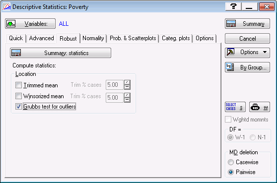
To perform this test, return to the Descriptive Statistics dialog box and select the Robust tab. This tab contains options for including  trimmed means, Winsorized means, and Grubbs test statistic in the Descriptive Statistics spreadsheet. Grubbs test for outliers (Grubbs 1969; Stefansky 1972) can be used to detect a single outlier at a time. It works by quantifying how far the suspected outlier is from other data points. Grubbs test statistic (G) is calculated as the ratio of the largest absolute deviation from the sample mean to the sample standard deviation.

On the Robust tab, select the Grubbs test for outliers check box.

Now click the Summary: statistics button to generate a spreadsheet that contains descriptive statistics for all variables.

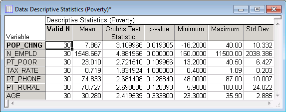
Here, we can see that the Grubbs Test Statistic for N_EMPLD is 4.88. It has a p-value of 0.00. This small p-value is evidence that there is at least 1 outlier in the N-EMPLD variable.

Select the original Poverty.sta data file.

STATISTICA provides a "data cleaning" facility that can be used to recode outliers. To access this feature:

Ribbon bar. Select the Data tab; in the Transformations group, click the Filter/Recode arrow and select Recode Outliers.

Classic menus. Select Recode Outliers from the Data - Data Filtering/Recoding submenu.

In the Recode Outliers and Extreme/Rare values dialog box, click the Variables button. In the Select Variables dialog box, click the Select All button, and then click OK.

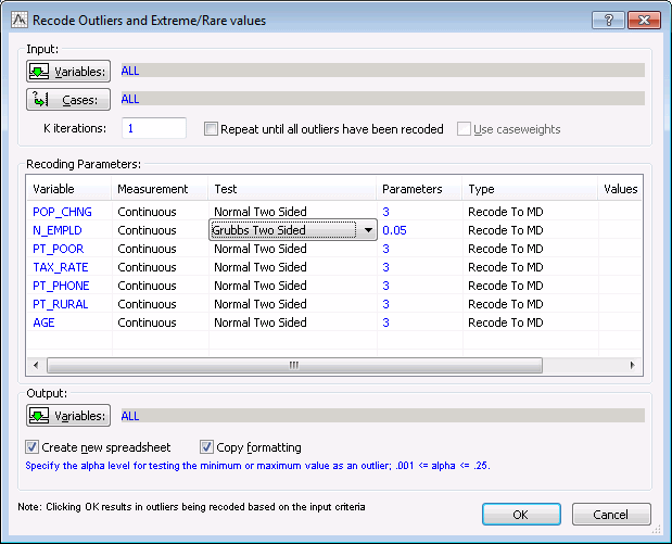
The Recode Outliers and Extreme/Rare values dialog box provides various tests for identifying outliers in continuous and categorical variables. For categorical variables, Statistica will treat as outliers those cases with codes or category values (text values) that occur with less than a specified relative frequency. For continuous variables, you can choose between a variety of tests including a Normal test, a Grubbs test, a Percentile test, and a Tukey test. All of these tests can be two-sided or one sided (directed to either the upper or lower end of the distribution).

For this example, set the Test cell for N_EMPLD to Grubbs Two Sided (click in the Test cell and select the desired test from the drop-down list) and set the Parameters cell to 0.05.

As mentioned previously, this facility also enables you to recode any identified outliers.

To do this, scroll to the right of the Recoding Parameters grid. In the Type column, you can choose from several recoding options: No Recode, Recode to MD (missing data), Recode to Value, Recode to Mean, Recode to Mode, Recode to Percentile, or Recode to Boundary. Depending on the type of recoding you select, you may need to enter a value (e.g., the percentile) in the Values column. Also, you can choose to apply case states (e.g., No Change, Label, Off, Marked, Cell Marked) to the identified outlier.

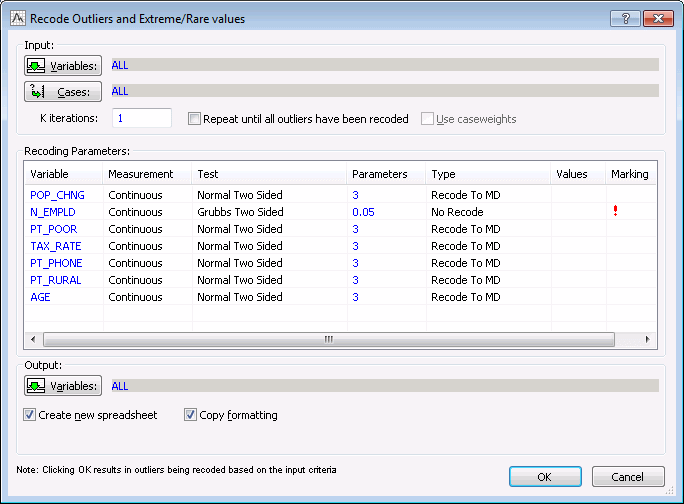
For this example, let's assume that we do not want to recode the outlier. Instead we want to mark it in the spreadsheet so that we can determine if it needs to be recoded.

In the N_EMPLD row, set the Type column to No Recode, and then single-click in the Marking cell and select Marked from the drop-down list. The dialog box should look as shown below.

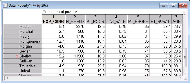
By default, Statistica will create a new spreadsheet that contains all the variables in the current spreadsheet. You can change these settings using the options in the Output group box, but for this example the default settings are fine. Click OK to create the new spreadsheet.

Scroll down in the spreadsheet, and you will see that the county of Shelby has 11,500 people employed in agriculture. This is a much greater number than is reported for other counties.

For more information on outliers, see Outliers, Correlations Introductory Overview - Outliers, and Quantitative Approach to Outliers.

For examples that further explore the Poverty.sta data set, see Multiple Regression Example 1: Standard Regression Analysis, GLM Example 7: Simple Regression Analysis, GLM Example 8: Multiple Regression Analysis, PLS Example 1: Multiple Regression, GC&RT Example 2: Regression Tree for Predicting Poverty, Boosting Trees Example 2: Prediction of Continuous Dependent Variable, Interactive Trees (C&RT, CHAID) Example, Example: Goodness of Fit Indices for Regression Predictions, MARSplines Example, Support Vector Machine Example 2 - Regression, and Example: Regression Random Forests.