Example 2: Analyzing Power, Sample Size, and Effect Size in 1-Way ANOVA
The standard approach to statistical testing, power and sample size analysis in the 1-Way Analysis of Variance (ANOVA), presented in virtually all textbooks, is centered around the hypothesis testing approach. Statistica Power Analysis is compatible with this traditional approach, but the program goes considerably beyond this approach by implementing advanced confidence interval estimation procedures, post hoc statistical estimation of power and required sample size, and non-standard hypothesis testing. With these advanced methods, you are in a better position to avoid some of the controversies and fallacies inherent in the more traditional approach (See, e.g., Cohen (1994), Schmidt & Hunter (1997).
To begin, let's perform a standard power and sample size analysis. Imagine you are planning to perform a 1-Way ANOVA to examine the effect of a new drug that is an improved version of a drug you tested approximately a year ago. The key questions are, what kind of statistical power is it reasonable to expect, and what kind of sample size is necessary to achieve a level of power that makes the experiment worth performing.
Specifying baseline parameters
Ribbon bar. Select the Statistics tab. In the Advanced/Multivariate group, click Power Analysis to display the Power Analysis and Interval Estimation Startup Panel.
Classic menus. From the Statistics menu, select Power Analysis to display the Power Analysis and Interval Estimation Startup Panel.
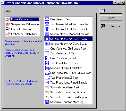
In the Startup Panel, select Power Calculation and Several Means, ANOVA, 1-Way.
Now, click the OK button to display the 1-Way ANOVA: Power Calc. Parameters dialog box.
Statistica can handle power analysis for two distinctly different kinds of models. The more familiar model, Fixed Effects, restricts you to making inferences about the actual treatments that are included in the experiment. The Random Effects model assumes you have randomly sampled your treatment levels from some larger population of levels. In this case, you can make inferences about the variation in the entire population of potential treatments.
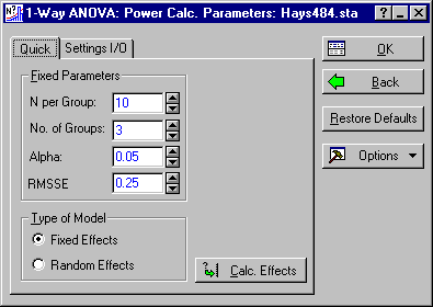
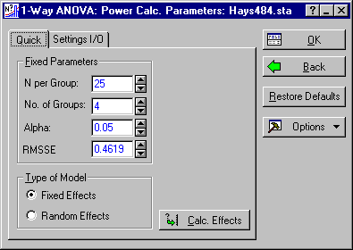
Assume in this case that we are operating with a Fixed Effects model. In order to calculate power, we need to specify the Fixed Parameters shown on the
Quick tab. Suppose we are planning to have four groups in the experiment, and we are anticipating using the traditional value of
![]() = .05 as our significance level. To begin with, we might anticipate using 25 subjects per group, because that is the sample size employed in the testing on the previous drug. Hence, enter 25 in the N per Group box, 4 in the No. of Groups box, and .05 in the Alpha box.
= .05 as our significance level. To begin with, we might anticipate using 25 subjects per group, because that is the sample size employed in the testing on the previous drug. Hence, enter 25 in the N per Group box, 4 in the No. of Groups box, and .05 in the Alpha box.
- Effect Size In 1-Way ANOVA
- The final number to be entered in the Fixed Parameters group is the RMSSE, which is a measure of the size of standardized effects in the design. In 1-Way ANOVA, with the other parameters held constant, power is a function of the noncentrality parameter
 which is a simple function of sample size, and the variation among the sample means. One possible way of characterizing
 is in relation to a quantity we call the Root Mean Square Standardized Effect, or RMSSE. This quantity is the sum of squared standardized effects, divided by the number of effects that are free to vary in the experiment. Because effects in the 1-Way ANOVA are restricted to sum to zero (to achieve identifiability), there are actually only J - 1 free effects in a J group design. Dividing the sum of squared standardized effects by J - 1, then taking the square root gives the RMSSE. Dividing instead by J and taking the square root gives a similar measure called f. For an extensive discussion of the relationship between f and other related quantities such as
 2, the proportion of population variance accounted for by the treatment effects, see Cohen (1983, Chapter 8).
It is important to recognize that the RMSSE does not change if you add or subtract a constant from all group means in the analysis. But because the RMSSE, f, and related indices combine information about several treatments into a single number, it is difficult to assign a single value of any of these indices that is uniformly valuable as in index of "strong," "medium," or "weak" effects. To understand better why this is true, let's calculate the RMSSE for a typical 4-group experiment.
At this point, the 1-Way ANOVA: Power Calc. Parameters - Quick tab should look as follows.
Click the Calc. Effects button, to display the ANOVA Effects Calculation dialog box.
In this dialog box, you enter the common population standard deviation
 in the Sigma field. The default value for Sigma is 1, because if you choose to express the means in standard deviation units, then Sigma is arbitrary, and is set equal to 1. To see why this is true, set Sigma to 15, and enter 0, 15, 30, and 45 as the four Group Means.
Notice how, as you enter Group Means, the Effect Measures, RMSSE and f, are recalculated automatically. In terms of the standard deviation, the means are 0, 1, 2, and 3 standard deviation units.
Now, change Sigma back to 1, and enter 0, 1, 2, and 3 as the Group Means. Notice that the f and RMSSE values are identical to the previous values.
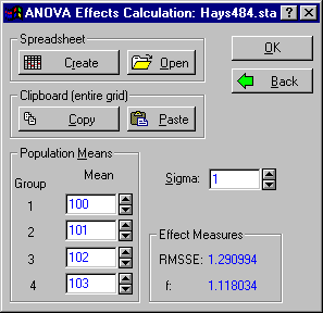
Now add 100 to each of the four Group Means.
Notice that the Effect Measures still have not changed. The Effect Measures are said to be invariant under linear transformations of the Group Means.
Since, in many cases, the standard deviation, and overall average of the group means represent arbitrary scale factors, we encourage you to think in "standardized effect units" about your group means. However, there are some situations where effects conceptualized more conveniently in commonly employed units, so there are obvious exceptions to this preference.
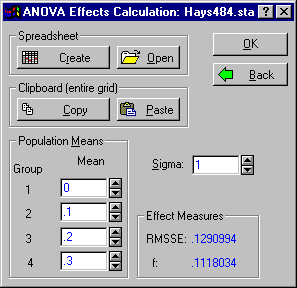
Suppose that, in our hypothetical drug experiment, the first group represents a placebo control, i.e., a group effect of 0, and that the remaining three groups represent three uniformly increasing levels of the drug. Suppose further that each increase in the drug causes an increase of .1 standard deviations, i.e., a small effect. Then the group means would appear as shown below.
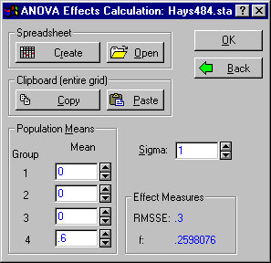
Notice that there are three groups in which the drug is administered, and that the average effect, in the substantive sense, is .2 for the three treatments (i.e., (.1 + .2 + .3)/3). However, the Effect measures do not fully reflect the size of the experimental effects in the analysis, because in the analysis of variance, effects are restricted arbitrarily to sum to zero. So the effects for the four groups are -.15, -.05, +.05, and +.15, respectively. This distinction between effects in the experimental sense, and effects as they are formally defined in ANOVA, is not always emphasized in standard textbook treatments. Yet, proper consideration of the issue raises some interesting dilemmas. Consider another experiment, in which three different drugs are compared to a placebo control, and imagine that two of the treatments have no effect, while the third treatment has an effect of .6 standard deviation units. Enter the values for this hypothetical experiment in the dialog as shown below.
Note: while the average effect of the drugs is .2 standard deviations, just as in the previous experiment, the effect measures are much larger in this experiment. Because the effect measures that relate to power are a measure on the variance of the group means, and because the variance carries several numbers into one, there cannot be a uniform standard for translating notions of "small," "medium," and "large" experimental effects into an f or RMSSE value.There are tentative suggestions by authors such as Cohen (1983), who designated f values of .1, .25, and .40 as representing "small," "medium," and "large" effects. Some readers seem to believe that these suggestions represent important rules of thumb, but it seems clear that they are little more than rough guidelines, and that proper power analysis should examine a range of values, perhaps ranging around Cohen's guidelines. When using the RMSSE, we suggest comparable rough guidelines of .15, .3, and .5 for "small," "medium," and "large" effects.
Of course, if your research is strictly exploratory, the cell means and/or effect size that you specify are strictly hypothetical. In a subsequent section, we will learn how to use statistical information from a previous study to make informed judgments about effect size.
Suppose we use Cohen's guideline for a "medium" effect size. Since
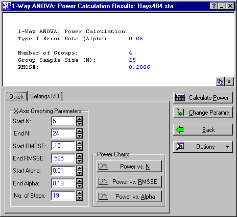
Cohen's guideline (an f of .25) corresponds, when J = 4, to an RMSSE of .2886. Click the OK button on the ANOVA Effects Calculation dialog box to return to the 1-Way ANOVA: Power Calc. Results - Quick tab and then enter .2886 in the RMSSE box.
Click the OK button to proceed to the 1-Way ANOVA: Power Calculation Results dialog box.
- Graphical Analysis of Power
- The
1-Way ANOVA: Power Calculation Results - Quick tab contains a number of options for analyzing power as a function of effect size, Alpha, or N.
Click the Calculate Power button to display a spreadsheet with power calculated for the currently displayed fixed parameters.
In this case, we see that, for "medium" size effects, power is simply inadequate for a sample size of 25.
On the 1-Way ANOVA: Power Calculation Results - Quick tab, change the Start N to 25 and the End N to 100, to provide a wide range of values.
Then click the Power vs. N button to produce a power chart.
The chart shows that power accelerates rather smoothly as N increases from 25 to 50, and then starts to level off. Power of .80 can be achieved with a sample size of approximately 45.
An important question is how sensitive the results displayed above are to the size of the experimental effects in the ANOVA design. For example, if effects satisfy Cohen's guideline for "large," (f = .4, RMSSE = .4619), how much impact will that have on power?
Click the Change Paramrs button to return to the 1-Way ANOVA: Power Calc. Parameters dialog box, and change the RMSSE value to .4619.
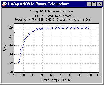
Click the OK button, and again click the Power vs. N button on the 1-Way ANOVA: Power Calculation Results - Quick tab.
Clearly, the difference between "medium" and "large" effects has an overwhelming effect on power. Merging the graphs (via the Graph Data Editor) and adding legends (via the Plots Legend command selected from the Insert menu) gives an even clearer picture.
An alternative approach is to fix N at, say, 25 and examine the relationship between power and RMSSE. Therefore, click the Power vs. RMSSE button on the 1-Way ANOVA: Power Calculation Results - Quick tab.
This graph shows that, with a sample size of 25 per group, it makes a very substantial difference whether RMSSE is in the range of .3 or .5. There is an important lesson here. Remember that, in the preceding discussion of how RMSSE, f, and similar measures were computed, we discovered that, depending on how they are distributed, a similar set of experimental effects may generate substantially different "ANOVA effects," and consequently may produce differences in power. It is not the size of effects, per se, that the ANOVA F-statistic is sensitive to, but rather the variation in effects (or, equivalently, the variation in group means). So when planning a study, you should choose a sample size that guarantees respectable power across a reasonable range of RMSSE values.
- Graphical Analysis of Sample Size
- Suppose you are anticipating "medium" effects, corresponding to an RMSSE of roughly .3. To be on the safe side, and allow for error in your estimate of effect size, it might be wise to examine the sample size required to produce your target power (or Power Goal) for a range of RMSSE values centered on .3. Click the Back button in both the
1-Way ANOVA: Power Calculation Results and the
1-Way ANOVA: Power Calc. Parameters dialog boxes to return to the Startup Panel. Here, select Sample Size Calculation and Several Means, ANOVA, 1-Way.
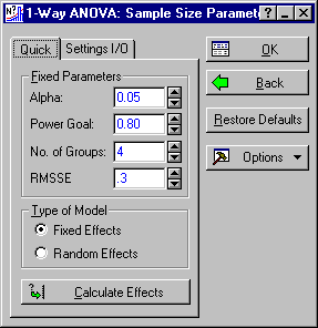
Click the OK button to display the 1-Way ANOVA: Sample Size Parameters dialog box. Enter the Fixed Parameters for the analysis as shown below.
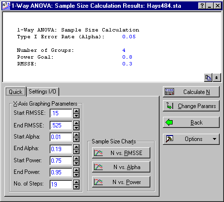
Then click the OK button to display the 1-Way ANOVA: Sample Size Calculation Results dialog box.
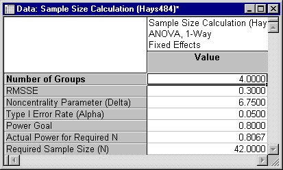
Click the Calculate N button to calculate the required sample size.
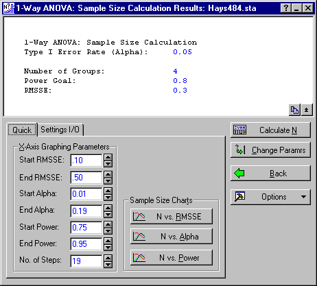
You can see that an N of 42 generates power slightly greater than the Power Goal of .80. Next, produce a graph showing the values of N required to generate a power of at least .80 for a range of RMSSE values from .10 to .50. Enter these RMSSE values in the Start RMSSE and End RMSSE boxes under X-Axis Graphing Parameters on the 1-Way ANOVA: Sample Size Calculation Results - Quick tab, as shown below.
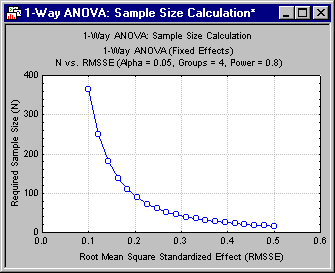
Click the N vs. RMSSE button to produce the following graph.
The graph shows, quite clearly, that required sample size is a rather linear function of RMSSE for RMSSE values ranging from .3 to .5, but that as RMSSE drops below .2, the required sample size accelerates upward at an alarming pace. Clearly, in this situation, whether effects are small or large has a massive effect on required sample size. By simply altering the values of Start RMSSE and End RMSSE, you can focus on any range of the graph that interests you. For example, below is the graph of required N for RMSSE values ranging from .2 to .4. You can see that, even in this rather narrow range of effect sizes, RMSSE has a powerful effect on the required N.
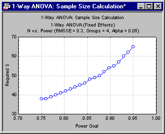
You can also examine the effect of Power Goal on the required N. Set a range of values to explore by adjusting the Start Power and End Power values under X-Axis Graphing Parameters. Then click the N vs. Power button to produce the graph. Below, for example, is a graph of Required Sample Size N versus Power Goal, for values ranging from .75 to .95.
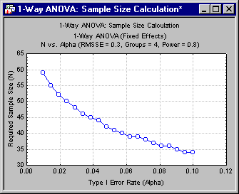
You can also graph the relationship between N and alpha. Below is a graph demonstrating the relationship for values of alpha ranging from .01 to .10. (Enter .01 in the Start Alpha box and .10 in the End Alpha box, and then click the N vs. Alpha button.)
Noncentrality-based interval estimates of effect size
With Statistica Power Analysis, you can compute, on the basis of an observed F, confidence intervals on the RMSSE and related quantities. Perhaps unnoticed by some is that these confidence intervals can be employed to test a wide range of nonstandard hypothesis tests in the analysis of variance.
A growing number of authors, in a wide range of contexts, have pointed out the logical flaws inherent in testing hypotheses of "null effect." Cohen (1994) in a very general but particularly influential article, suggested that confidence interval estimates, and estimates of effect size, would be important improvements on current practice of testing the "nil hypothesis," i.e., a hypothesis of zero effect. Cohen (1994) gave no technical details about how this idea might be implemented.
There are two fundamental approaches to dealing with the logical problems inherent in testing the "nil hypothesis." One approach is to test a relaxed version of the null hypothesis. For example, consider the 1-Way ANOVA. The traditional F-test is actually a test that, in the population, the RMSSE is equal to zero. The relaxed version of this procedure is to pick a more reasonable target value. For example, you might pick a trivial value of the RMSSE (say .10) and test the hypothesis that, in the population, the RMSSE is less than or equal to this trivial value. Rejection of this hypothesis would imply a nontrivial effect.
Replacement of the test of zero effect with a test of trivial effect has been suggested by a number of authors. (Serlin & Lapsley, 1985, 1993; Browne & Cudeck, 1992; Murphy & Myors, 1998). Although this approach offers definite advantages, there are a number of problems connected with it. In particular, any hypothesis test, whether it be a test of a zero effect or a hypothesis of trivial effect must be performed with proper control of Type I error and power.
Moreover, a cutoff value for triviality must be specified. Not only are such values controversial, but as our previous discussion has emphasized, the same value of RMSSE (or related quantities such as
 2) may have somewhat different interpretations in different situations.
The emphasis on hypothesis testing is so deeply embedded in modern science that many apparently have failed to notice that confidence interval procedures offer all the advantages of tests of trivial effect, and more. For example, all tests of trivial effect, regardless of the cutoff value, can be performed simply by examining the confidence interval for RMSSE. For example, the hypothesis test of the hypotheses
can be performed simply by observing whether an appropriate confidence interval excludes .10. (More about that below.) However, the confidence interval contains more information than that provided by the hypothesis test or its associated p-value, because the width of the confidence interval provides information about how precisely the population RMSSE has been determined on the basis of the sample data. For an extensive discussion of this point, with numerical examples, see Steiger & Fouladi (1997).
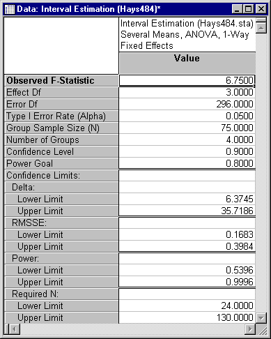
Suppose, for example, a four group ANOVA, with 75 subjects per group, has been performed, and an F value of 6.75 has been observed. What has been learned about the actual population effects in this experiment?
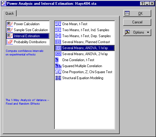
Click the Back button on both the 1-Way ANOVA: Sample Size Calculation Results and the 1-Way ANOVA: Sample Size Parameters dialog boxes to return to the Startup Panel. Here, select Interval Estimation and Several Means, ANOVA, 1-Way.
Click the OK button to display the 1-Way ANOVA: Interval Estimation dialog box.
Enter the data as shown below on the 1-Way ANOVA: Interval Estimation - Quick tab.
Click the Compute button to compute several interesting confidence intervals.
The first confidence limits shown are for the noncentrality parameter
 . (This can be useful to advanced users who wish to compute confidence intervals on functions of
 .)
.)
Next is the set of confidence limits for the RMSSE. In this case, the limits extend from .1683 to .3984. This demonstrates that, even with this reasonably large sample size, there is a fair range of uncertainty. Note however, that one could reject the hypothesis that effects are trivial (see Equation 3 above) at the .05 significance level, because the 90% confidence interval excludes the value .10. In a similar vein, we could use the confidence interval to test the hypothesis that the effects are more than strong. If we use an RMSSE cutoff value of .50 to define "strong" effects, the null hypothesis that effects are strong is
Since, in this case, the confidence interval does not include the value .50, we can reject the hypothesis that effects are strong at the .05 level. In other words, we know that effects are not trivial, and they are not strong. They are somewhere in between.
See also, Power Analysis - Index.

