Example 10.1: Constructing a Simple D-Optimal Design
- Overview
- The notion of D- and A-optimal designs is discussed in the Introductory Overview. In short, from a set (candidate list) of valid experimental points (i.e., settings of factors in the study), we can select the best (fixed) number of points so as to maximize the amount of information that can be extracted from the experimental region. In principle, we want to extract the points so that the factor effects in the final design are orthogonal (independent), or close to orthogonal.
For example, consider a simple 32 factorial design. If we wanted to fit to the data (which we intend to collect later) a simple first-order linear main effects model, we really only need to select the extreme values for each factor, since no information about those linear effects is added by including the center point values for each factor. Thus, we would select the points that would define a 22 factorial design. However, if we intend to fit a second-order (quadratic) model, we need the center point values so that we can estimate the quadratic components. In this example, how the D-optimal search algorithms will follow exactly this logic will be demonstrated.
Specifying a Simple 32 Design. First let's generate the simple complete 3 by 3 design. Start the Experimental Design (DOE) analysis:
Ribbon bar. Select the Statistics tab, and in the Industrial Statistics group, click DOE to display the Design & Analysis of Experiments dialog box.
Classic menus. On the Statistics - Industrial Statistics & Six Sigma submenu, select Experimental Design (DOE) to display the Design & Analysis of Experiments dialog box.
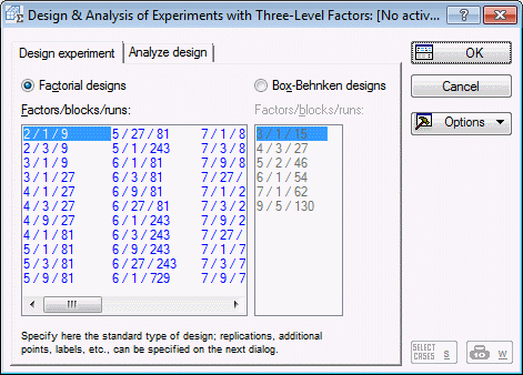
On the Quick tab, select 3**(K-p) and Box-Behnken designs and click the OK button.
In the Design & Analysis of Experiments with Three-Level Factors dialog box, the default design is selected: 2/1/9 (2 factors, 1 block, 9 runs).
Click OK.
In the Design of an Experiment with Three-Level Factors dialog box, on the Quick tab, select the Standard order option button. Then, click the Summary: Display design button to produce the design in a spreadsheet.
We can now save this design, and close all dialog boxes and spreadsheets.
- Specifying the candidate list
- Now, open the example data file 3x3.sta:
Ribbon bar. Select the Home tab. In the File group, click the Open arrow and on the menu, select Open Examples to display the Open a Statistica Data File dialog box. Open the 3x3.sta data file, which is located in the Datasets folder.
Classic menus. On the File menu, select Open Examples to display the Open a Statistica Data File dialog box. Open the 3x3.sta data file, which is located in the Datasets folder.
Start the Experimental Design analysis again.
In the Startup Panel, select the Advanced tab. Select D- and A- (T-) optimal algorithmic designs and click OK to display the D- and A-Optimal Designs dialog box.
First, we need to enter a candidate list of points, that is, the list of points from which we want Statistica to construct the design.
Click the Variables button, and in the variable selection dialog box, select both variables. Click the OK button.
In the D- and A-Optimal Designs dialog box, click the Display and modify candidate points button to display the List of Candidate Points for Optimal Design.
Note: here we can modify these values, or force particular points into the final design. This option is particularly useful when we have already collected data for the dependent variable for some runs in the design. By forcing those existing points into the final design, we can in effect repair or enhance an existing design. In this case, however, simply click OK to accept the points as they are. - Specifying the first-order design
- First, we will select points so as to maximize the information for a first-order, Linear main effects model. This is the default model, selected on the
Model tab, so simply click OK. After a few iterations with the default search method [Sequential (Dykstra)], the
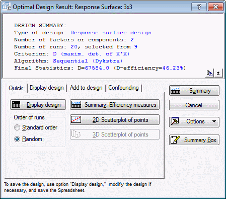
Optimal Design Result: Response Surface dialog box will be displayed.
As you can see in the summary box, the D-efficiency of the chosen design (20 points) is 100%. This measure can be interpreted as the relative number of runs (in percent) that would be required by an orthogonal design to achieve the same value of the determinant |X'X| (where X is the design matrix; see also the Introductory Overview). Apparently, the chosen design is an orthogonal design.
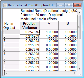
On the Quick tab, click the Display design button to review the selected points.
Only the first several points are shown in the spreadsheet above. Clearly, and as expected, Statistica has chosen only the extreme points (only those where the factor settings were either high or low) from the list of candidates. (See Optimal Design Result: Response Surface - Quick tab for an explanation of the values in the Prediction Variance column.) Thus, in effect, this design is a replicated 22 factorial design.
- Specifying the second-order design
- Now return to the
Optimal Design Result: Response Surface dialog box, and click Cancel to display the
D- and A-Optimal Designs dialog box again.
Select the Model tab, and select the Lin/quad. main effects option button to specify a model that includes the nonlinear (squared) factor effects in the model. Click OK.
Now the D-efficiency is less than 100%. However, note that the values for the D-efficiency measure should be interpreted only relative to other similar designs (see the Introductory Overview). Next, click the Display design button.
As expected, Statistica has chosen not just points with extreme value settings for the two factors, but also points with intermediate factor settings. Otherwise, a quadratic model could, of course, not be fitted to the data.
See also, Experimental Design.


