Conceptual Overviews - Bivariate Histograms
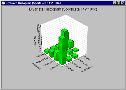
Three-dimensional (bivariate) histograms are used to visualize crosstabulations of values in two variables. They can be considered to be a conjunction of two simple (i.e., univariate) histograms, combined such that the frequencies of co-occurrences of values on the two analyzed variables can be examined.

There are two major reasons why frequency distributions (either univariate or bivariate, such as those visualized in 3D histograms) are of interest.
• One can learn from the shape of the distributions about the nature of the examined variables (e.g., a bimodal distribution may suggest that the sample is not homogeneous, and consists of observations that belong to two populations that are more or less normally distributed); this application is particularly relevant for smoothed 3D Bivariate Histograms (see below).
• Many statistics are based on assumptions about the distributions of analyzed variables; 3D Bivariate Histograms help one to test whether those assumptions are met for pairs of variables.
3D Histograms vs. Crosstabulations
3D Bivariate Histograms provide information similar to crosstabulations. Although specific (numerical) frequency data are easier to read in a table, the overall shape and global descriptive characteristics of bivariate distributions may be easier to explore in a graph. Moreover, the graph provides qualitative information about the distribution that cannot be fully represented by any single index. For example, a bivariate skewed distribution of response latencies vs. the duration of a reaction-time task (in a reaction-time experiment) may result from the changes in subjects' strategies of dealing with fatigue.
Different Categorization Methods in One Graph
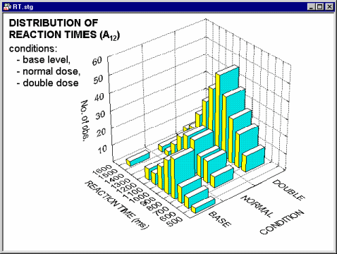
Different methods of categorization can be used for each of the two variables for which the bivariate distribution is visualized in the graph, as illustrated in the following 3D Bivariate Histogram of reaction time scores by experimental condition.

Specifically, in this graph the distribution of reaction times (a continuous variable categorized by dividing the entire range of values into 12 intervals of equal size) can be reviewed across three experimental conditions (a discrete variable with three distinctively labeled levels: BASE, NORMAL, and DOUBLE).
- Smoothing Bivariate Distributions
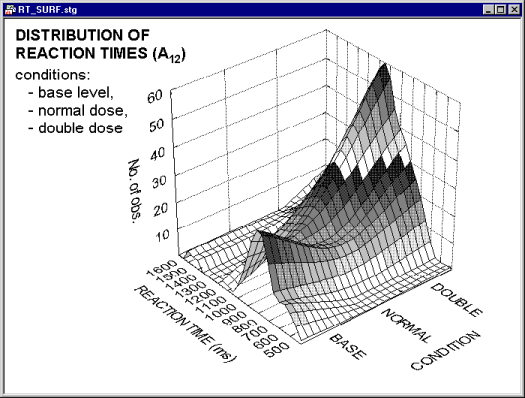
- The smoothing facilities available for 3D Bivariate Histograms allow you to fit surfaces to 3D representations of bivariate frequency data. Thus, every 3D histogram can be turned into a smoothed surface. This technique is of relatively little help if applied to a simple pattern of categorized data (such as the histogram that was shown above).

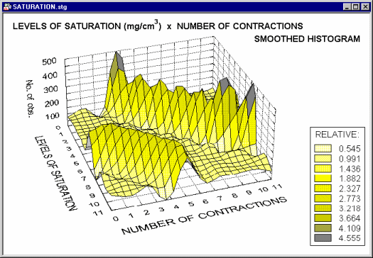
However, if applied to more complex patterns of frequencies, it may provide a valuable exploratory technique,

allowing identification of regularities which are less salient when examining the standard 3D histogram representations (e.g., see the systematic surface "wave-patterns" shown on the smoothed histogram above).
