SANN Example 1: Performing Regression with 4-Bar Linkage Data
Overview: This example illustrates the method to perform regression analysis using Statistica Automated Neural Networks (SANN). In particular, it describes how to choose and retain models using novel, state-of-the-art algorithms capable of ranking alternative models based on performance and suitability for the given task according to user-defined search criteria and configurations.
This example is based on a data set describing the dynamics of the 4-bar linkage. The goal of the project is to create a neural network model architecture that can best describe the relationship between the target and input variables that drive and control the behavior of the mechanical system.
The example concentrates on data modeling using the Statistica Automated Network Search (ANS), although the choice of the Custom Neural Network (CNN) strategy is also possible.
As you work through the example, you may find it necessary to read through the Neural Networks Overviews, which contain an introduction to the basic concepts of neural networks and include a list of references to good introductory textbooks.
Purpose: The purpose of this example is to illustrate the adeptness of the Automated Network Search application with regard to modeling data that are nonlinear in nature.
Problem definition: The problem is to find a neural network architecture that accurately relates the targets of the 4-bar example to the input variables. This process involves training a finite set of neural network architectures and retaining the one that is best suited for the task given a number of user-defined search criteria and conditions.
Data set:
The data set contains a sample of the so called 4-bar linkage (see schematic above). The figure shows the main variables of the physical model, including the 4-bar lengths R1, R2, R3, R4, and the angle T2 as the input variables, and four target variables T3, T4, H1, and V1. The targets are related to the inputs via the following equations:
As the above equations indicate, the relationships between the input and target variables are highly nonlinear. Automated Network Search (ANS) looks for the underlying trend that accurately relates every instance of the targets to the corresponding instance of inputs. Note that, in addition to the target variables T3, T4, H1, and V1, there is also the intermediate angle variable
![]() , which can be summarized as a function of R1, R2, R3, R4, and T2. Every target variable is then expressed as a function of
, which can be summarized as a function of R1, R2, R3, R4, and T2. Every target variable is then expressed as a function of
![]() in closed form. In this example, however, we use the primary input variables instead of
in closed form. In this example, however, we use the primary input variables instead of
![]() .
.
We model the above variables using the Automated Network Search (ANS) to relate the target variable to the inputs.
This example explains performing regression with 4-bar linkage data.
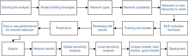
Starting the analysis
- Ribbon bar. Select the Home tab. In the File group, click the Open arrow and from the menu, select Open Examples. The Open a Statistica Data File dialog box is displayed. 4bar linkage.sta is located in the Datasets folder.
- Classic menus. From the File menu, select Open Examples to display the Open a Statistica Data File dialog box; 4bar linkage.sta is located in the Datasets folder.
A portion of the data is shown below.
- Ribbon bar: Select the Data Mining tab. In the Learning group, click Neural Networks to display the SANN - New Analysis/Deployment Startup Panel. Or, select the Statistics tab. In the Advanced/Multivariate group, click Neural Nets to display the SANN - New Analysis/Deployment Startup Panel.
- Classic menus: From the Statistics menu or the Data Mining menu, select Automated Neural Networks to display the SANN - New Analysis/Deployment Startup Panel.
-
For this example, select Regression in the New analysis list.
- Click the OK button to display the SANN - Data selection dialog box, which contains options to specify the training, testing, and validation subsets and the variables to use in the analysis. We will also select our strategy for the analysis.
- On the Quick tab, click the Variables button to display a standard three-variable selection dialog box. For Continuous targets, select T3, T4, H1, and V1, and for the Continuous inputs select the primary input variables R1, R2, R3, R4, and T2.
- Click OK to accept the variable selections, close the dialog box, and return to the SANN - Data selection dialog box.
- Select the Sampling (CNN and ANS) tab. The performance of a neural network is measured by how well it generalizes to unseen data (that is, how well it predicts data that was not used during training). The issue of generalization is actually one of the major concerns when training neural networks. When the training data have been overfit (that is, been fit so completely that even the random noise within the particular data set is reproduced), it is difficult for the network to make accurate predictions using new data.
- One way to combat this problem is to split the data into two (or three) subsets: a training sample, a testing sample, and a validation sample. These samples can then be used to 1) train the network, 2) verify, or test, the performance of the networks as they are trained, and 3) perform a final validation test to determine how well the network predicts new data.
- In SANN, the assignment of the cases to the subsets can be performed randomly or based upon a special subset variable in the data set. The 4bar linkage.sta file already contains a subset variable that splits the data into two subsets. We will use this variable to specify a training subset and a testing subset.
- On the Sampling (CNN and ANS) tab, select the Sampling variable option button, and click the Training sample button to display the Sampling variable dialog box.
- Click the Sample Identifier Variable button to display a variable selection dialog box. Select Subset and click the OK button.
- Subset contains two codes – Train and Validation – which can be seen by double-clicking in the Code for training sample field to display the Variable code dialog box.
- For the training sample, select Train and click OK to close this dialog box and return to the Sampling variable dialog box. Select the On option button in the Status group box. The dialog box should look as follows.
- Click OK to return to the SANN - Data selection dialog box.
- Click the Testing sample button, and specify the variable and code for the testing subset. Remember to set the Status to On. The dialog box should look as follows.
- After specifying the variable and code, click OK to return to the SANN - Data selection dialog box. The variable and code for each sampling subset is shown adjacent to the appropriate button.


Model building strategies
SANN provides three neural network search strategies that can be used in generating your models: Automated Network Search (ANS), Custom Neural Networks (CNN), and Subsampling (random, bootstrap). The ANS facility is used for creating neural networks with various settings and configurations while requiring minimal specifications from you. ANS helps you create and test neural networks for your data analysis and prediction problems. It designs a number of networks to solve the problem and then selects those networks that best represent the relationship between the input and target variables (that is, those networks that achieve the maximum correlation between the targets and the outputs of the neural network).
The Custom Neural Networks (CNN) tool enables you to choose individual network architectures and training algorithms to exact specifications. You can use CNN to train multiple neural network models with exactly the same design specifications but with different random initialization of weights. As a result, each network finds one of the possible solutions posed by neural networks of the same architecture and configurations. In other words, each resulting network provides you with a suboptimal solution (that is, a local minimum).
The Subsampling (random, bootstrap) tool enables you to create an ensemble of neural networks based upon multiple subsamples of the original data set. Options for this strategy are available on the Subsampling tab.
To select a strategy, select the Quick tab of the SANN - Data selection dialog box. For this example, select the Automated network search (ANS) option button located in the Strategy for creating predictive models group box, and then click the OK button to display the SANN - Automated Network Search (ANS) dialog box.
Before training our networks, let's review some of the options that are available in this dialog box.
Network types
The ANS can be configured to train both multilayer perceptron (MLP) networks and radial basis functions (RBF) networks. The multilayer perceptron is the most common form of network. It requires iterative training, which may be slow, but the networks are quite compact, execute quickly once trained, and in most problems yield better results than the other types of networks. Radial basis function networks tend to be larger than multilayer perceptron, and often have worse performance. They are also usually less effective than multilayer perceptrons if you have a large number of input variables (they are more sensitive to the inclusion of unnecessary inputs). Also, RBF networks are not particularly suitable for modeling data with categorical inputs since the basis functions of RBF reside in a continuous space while categorical inputs are discrete by nature.
Network complexity
One particular issue you need to observe is the number of hidden units (network complexity). For example, if you run ANS several times without producing any good networks, you may want to consider increasing the range of network complexity tried by ANS. Alternatively, if you believe that a certain number of neurons is optimal for your problem, you can then exclude the complexity factor from the ANS algorithm by simply setting the Min. hidden units equal to the Max. hidden units. This way you will help the ANS to concentrate on other network parameters in its search for the best network architecture and specifications, which unlike the number of hidden units, you do not know a priori. Note that network complexity is set separately for each network type.
Networks to train, Networks to retain
The number of networks that are to be trained and retained can be modified on the Quick tab. You can specify any number of networks you want to generate (the only limits are the resources on your machine) and choose to retain any number of them when training is over. If you retain more than one network, you can use them for making predictions both as stand-alones and ensembles. Predictions of an ensemble of well-trained networks are generally more accurate as compared to the predictions of the individual members.
If you want to retain all the models you train, set the value in Networks to train equal to the Networks to retain. However, often it is better to set the number of Networks to retain to a smaller value than the number of Networks to train. This will result in SANN retaining a subset of those networks that perform best on the data set. The ANS is a search algorithm that helps you create and test neural networks for your data analysis and prediction problems. It designs a number of networks to solve the problem, copies these into the current network set, and then selects those networks that perform best. For that reason, it is recommended that you set the value in Networks to train to as high as possible, even though it may take some time for SANN to complete the computation for data sets with many variables and data cases and networks with a large number of hidden units. This configures SANN to thoroughly search the space of network architectures and configurations and select the best for modeling the training data.
MLP activation functions
Select the MLP activation functions tab to review the list of activation functions that are available for hidden and output layers of MLP networks. This tab is only visible when the MLP check box is selected in the Network types group box on the Quick tab.
Although most of the default configurations for the ANS are calculated from properties of the data, it is sometimes necessary to change these configurations to something other than the default. For example, you may want the search algorithm to include the Sine function (not selected by default) as a possible hidden and output activation function. This might prove useful when your data are radially distributed. Alternatively, you might know (from previous experience) that networks with Tanh hidden activations might not do so well for your particular data set. In this case, you can simply exclude this activation function by clearing the Tanh check box.
You can specify activation functions for Hidden neurons and Output neurons in an MLP network. These options do not apply to RBF networks. You can also restrict the ANS from searching for best hidden and output activation functions by selecting only one option among the many that are available. For example, if you set the choice of hidden activations to Logistic, the ANS then produces networks with this type of activation function only. However, you should generally only restrict the ANS search parameters when you have a logical reason to do so. Unless you have a priori information about your data, you should make the ANS search parameters (for any network property) as wide as possible.
Training the models
For this example, we leave all the options at their default values.
Now, click the Train button. During training, the Neural network training in progress dialog box is displayed, which provides summary details about the networks being built including the type of network, the activation functions, the training cycle, and the appropriate error terms.
After the training is completed, the SANN - Results dialog box is displayed. The Active neural networks grid (located at the top of the dialog box) displays the top five networks generated during the training. (See the note at the beginning of this topic about the results shown here being slightly different from your analysis.)
Reviewing the results
The SANN - Results dialog box provides a variety of options for generating predictions and graphs and for reviewing network properties. The Active neural networks grid at the top of the dialog box enables you to quickly compare the training and testing performance for each of the selected networks and provides additional summary information about each model including the algorithm used in training and the error function and activation functions used for the hidden and output layers. To generate a spreadsheet of the information in the Active neural networks grid, click the Summary button.

Predictions
In the SANN - Results dialog box, select the Predictions tab. The options on this tab can be used to generate a prediction spreadsheet for each of the networks retained during training or an ensemble (that is, a collection of neural networks that cooperate in performing a prediction). For this example, we want to look at the predictions of the first and second networks (note that your results will most likely vary from those shown here).
- Click the Select\Deselect active networks button, and in the Model activation dialog box, select the first and second models.
- Click OK to close this dialog box and return to the SANN - Results dialog box.
- On the Predictions tab, in the Predictions type group box, select the Standalones and ensemble option button.
- In the lower-right corner of the SANN - Results dialog box, in the Samples group box, select the Train and Test check boxes. When these check boxes are selected, the resulting spreadsheets will include cases from both the training sample and the testing sample.
- Click the Predictions button to generate Predictions spreadsheets for each of the four targets.
- This spreadsheet shows the predictions (output) for V1. Note that in addition to the predictions of the individual networks, the spreadsheet also contains (last column) the outputs of the ensemble, which is computed by simple averaging over the outputs of the standalone networks. It is highly recommended that you combine networks to form ensembles, especially when the size of the training set is small. Ensembles of well trained networks, in general, perform better than the individual members.

How to use the performance for network selection
SANN uses the correlation coefficient between the targets of the data and the outputs (predictions) of the network as a performance measure. The correlation coefficient measures how close the overall prediction of a network is to the target (dependent) data. The correlation coefficient can assume any value between -1 and 1, with 1 indicating a perfect fit. Since usually the target data consists of real measurements of one or more quantities of interest plus a certain amount of additive noise, a correlation coefficient close or equal to 1 measured on the training sample isn’t necessarily a desirable result (depending on the amount of noise present in the target variables). It actually could mean overfitting. When a network overfits the train data its correlation coefficient is maximum (that is, performs very well on the train sample). However, such networks usually perform badly on the test and validation samples. Therefore, you should always use the test and validation sample correlation coefficients for selecting networks. It should also be mentioned that just because the correlation coefficient is low doesn’t necessarily imply a badly trained network. In fact it could be a sign of a conservative network, which does its best to avoid fitting (modeling) the noise, which is necessary.
Graphs
- Select the Graphs tab of the SANN - Results dialog box. You can use the options on this tab to create histograms, 2D scatterplots, and 3D surface plots using targets, predictions, residuals, and inputs.
- For example, to review the distribution of the network residuals (that is, differences between the targets and their predicted values) of a target variable, say T3, select T3 from the Target variable drop-down list, and then select Residual in the X-axis list, and finally click the Histograms of X button.
- An examination of the histograms shows that the residuals are close to a normal distribution with a zero mean, which is a good indication that the network has discovered the assumed noise model (as with most neural network tools, SANN assumes that noise on the target variables is normally distributed with zero mean and an unknown variance). The larger the variance of the noise (that is, the more spread out the bins of the histogram), the larger the noise. A histogram width narrower than the true variance of noise is an indication of overfitting. However, the amount of noise (that is, its variance) is not known a priori.
- Another useful graph to review is the scatterplot of the observed and predicted values for the target variables. To do so, select Target in the X-axis list and Output in the Y-axis list, and click the X and Y button.
- You can use this graph to visually inspect how well a target is related to the network outputs by observing how close the graph is to the 45-degree line that is also displayed in the scatterplot. In fact, the graph is nothing more than a visualization of the correlation coefficient, which plays a central role in network selection. Note that most points of the scatterplot of the individual networks does not lie exactly on the 45-degree line. That is because the networks have recognized some noise on the target values and have avoided modeling them as true signals, which is a desired result.
Network details

Global sensitivity analysis
Global sensitivity analyses give you information about the relative importance of the variables used in a neural network. In sensitivity analysis, SANN tests how the neural network responses (predictions) and, hence, the error rates, would increase or decrease if each of its input variables were to undergo a change. In global sensitivity analysis, the data set is submitted to the network repeatedly, with each variable in turn replaced with its mean value calculated from the training sample, and the resulting network error is recorded. If an important variable changed in this fashion, the error increases a great deal; if an unimportant variable is removed, the error does not increase very much.
Click the Global sensitivity analysis button on the Details tab of the SANN - Results dialog box to conduct a global sensitivity analysis.
The spreadsheet shows, for each selected model, the ratio of the network error with a given input omitted to the network error with the input available. If the ratio is 1 or less, the network actually performs better if the variable is omitted entirely - a sure sign that it should be pruned from the network.
This is indicative of a limitation of sensitivity analysis. We tend to interpret the sensitivities as indicating the relative importance of variables. However, they actually measure only the importance of variables in the context of a particular neural model. Variables usually exhibit various forms of interdependency and redundancy. If several variables are correlated, then the training algorithm may arbitrarily choose some combination of them and the sensitivities may reflect this, giving inconsistent results between different networks. It is usually best to run sensitivity analyses on a number of networks, and to draw conclusions only from consistent results. Nonetheless, sensitivity analysis is extremely useful in helping you to understand how important variables are.
Local sensitivity analysis
The local sensitivity analysis is in many ways similar to the global sensitivity analysis, except that in the former we measure the change in the performance of neural networks due to changes induced to input values at arbitrary locations of the input space, i.e., in the vicinity of a point in the input space per variable. SANN measures local sensitivity for an input by varying the value of that input by an infinitesimal amount in 10 equally spaced individual points encompassed by the minimum and maximum of the train data, and then calculating the changes in the performance of the network as a result.
Although local sensitivity analysis should, in general, lead to the same conclusions about the importance of the inputs relative to the predictions of the neural network model. Nonetheless, the measures of local sensitivity may exhibit a kind of behavior that could only be interpreted on the basis of how important (influential) an input variable is ”at a given point in the input space.” For example, a network may be very sensitive to even minute changes in the value of an input at a certain region of the input space while that very same input remains unimportant elsewhere; i.e., large changes in the value of the input can yield little changes in predictions of the network.
Unique models, best models, good models
If you have not worked with neural networks for building predictive models, it is important to remember that these are ”general learning algorithms,” not statistical estimation techniques. That means that the models that are generated may not necessarily be the best models that could be found, nor is it necessarily true that there is a single best model. In fact, in practice, you will usually find several models that appear of nearly identical quality. Each model can be regarded, in this case, as a unique solution. Note that even models with the same number of hidden units, hidden and output activation function, etc., may actually have different, more or less, predictions and hence performance. This is due to the nature of neural networks as highly nonlinear models capable of producing multiple solutions for the same problem.
Deployment
With the SANN deployment options, you can quickly generate predictions from one or more previously trained networks based on information stored in industry-standard PMML (Predictive Model Markup Language) deployment code.
To save these two networks, click the Save networks button and select PMML from the drop-down list. In the Save PMML file dialog box, browse to where you want to save the files, enter 4barlinkage in the File name field, and click the Save button.
The two networks are saved as 4barlinkage-1.xml and 4barlinkage-2.xml. After you have saved the networks, close this analysis by right-clicking on the SANN - Results button on the analysis bar (located at the bottom of the Statistica window) and selecting Close.