Example 2: K-means Clustering
This example illustrates one other method of clustering: k-means clustering. As described in the Introductory Overviews, the goal of the k-means algorithm is to find the optimum "partition" for dividing a number of objects into k clusters. This procedure will move objects around from cluster to cluster with the goal of minimizing the within-cluster variance and maximizing the between-cluster variance. In Example 1, you identified three clusters in the car data set (Cars.sta), using the method of Joining (Clustering). Now you will see what kind of solution k-means clustering will suggest for 3 clusters.
Procedure
Specifying the Analysis
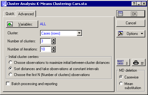
- Click the Advanced tab to further specify the analysis.
-
To view various result spreadsheets and plots for your analysis, click on the
Advanced tab .
Analysis of variance: In the K-means Clustering - Introductory Overview, k-means clustering was referred to as "analysis of variance in reverse". In an analysis of variance, the between-groups variance is compared to the within-groups variance to decide whether the means for a particular variable are significantly different between groups. Even though significance testing would not be proper in this case (you are very much capitalizing on chance), you may nevertheless look at the analysis of variance results, comparing the means for each dimension (that is, performance measure) between groups (clusters of cars). Click the Analysis of Variance button to display the Analysis of Variance spreadsheet.
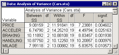
Judging from the magnitude (and significance levels) of the F values, variables Handling, Braking, and Price are the major criteria for assigning objects to clusters.
Identification of clusters
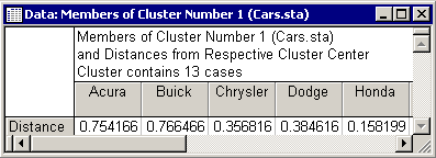
Now, see how STATISTICA assigned cars to clusters using these criteria. To view the members of each cluster, click the Members of each cluster & distances button to produce a cascade of spreadsheets (one for each cluster). Cluster 1 consists of Acura, Buick, Chrysler, Dodge, Honda, Mitsubishi, Nissan, Olds, Pontiac, Saab, Toyota, VW, and Volvo.
The next spreadsheet contains the members of Cluster 2:
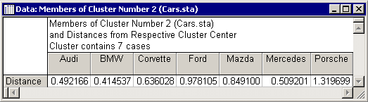
The second cluster contains Audi, BMW, Corvette, Ford, Mazda, Mercedes, and Porsche. The final cluster is given in the third spreadsheet. This cluster consists of Eagle and Isuzu.
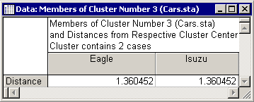
These results do not entirely match the clusters found in the previous analysis. However, the distinction between economy sedan vs. high luxury sedan still seems tenable. The Eagle and Isuzu were probably moved into their own category because they did not "fit" anywhere else, and because any other split between cars did not improve the solution (that is, increase between-groups sums of squares).
Descriptive statistics for each cluster
Another way of identifying the nature of each cluster is to examine the means for each cluster for each dimension. You can either display descriptive statistics separately for each cluster (click the Descriptive statistics for each cluster button), display the means for all clusters and the distances (Euclidean and squared Euclidean) between clusters in separate spreadsheet (click the Summary: Cluster means & Euclidean distances button), or plot those means (click the Graph of means button). Usually, the graph provides the best summary.
Looking at the lines for the economy sedan cluster (Cluster 1) as compared to the luxury sedan cluster (Cluster 2) it is found that, indeed, the cars in the latter cluster are:

The most distinguishing feature of the cars in the third cluster (Eagle and Isuzu) in this plot appears to be their shorter braking distances and their poorer handling.
Cluster distances: Other useful results to examine are the Euclidean distances between clusters (click the Summary: Cluster means & Euclidean distances button). These distances (Euclidean and squared Euclidean) are computed from the cluster means on each dimension.

Note that clusters 1 and 2 are relatively close together (Euclidean distance = 0.97) relative to the distance of cluster 3 from clusters 1 and 2.