Example 9.1: Finding Vertex and Centroid Points for a Constrained Region

A1x1 + A2x2 + ... + Aqxq + A0 ≥ 0

(where the A1s are weights, and the x1s denote the factor values) defines a line (or plane) through the experimental region; you can specify a practically unlimited number of such constraints, which Statistica will process one-by-one, to determine the vertex points resulting from the intersection of the constraint lines (planes). After all constraints have been processed, the program will then compute the respective centroids for each side of the (convex) hyperpolyhedron.

A: 0 <= xA <= 10

B: 0 <= xB <= 10

C: 0 <= xC <=10

In addition, 1) the values for factor A must be at least twice as large as those for factor B, and 2) the values for factor A and B combined must be greater than or equal to those for factor C:

(1) xA - 2*xB ≥ 0

(2) xA + xB - xC≥0

Ribbon bar. Select the Statistics tab, and in the Industrial Statistics group, click DOE to display the Design & Analysis of Experiments Startup Panel.

Classic menus. On the Statistics - Industrial Statistics & Six Sigma submenu, select Experimental Design (DOE) to display the Design & Analysis of Experiments Startup Panel.

Select the Advanced tab, select Designs for constrained surfaces and mixtures, and click the OK button to display the Design Points (Vertices & Centroids) for Constrained Surfaces and Mixtures dialog box.

The default number of factors is equal to 3, which you do not need to change for this example.

Let's first specify the factor minima and maxima. Click the Initial factor constraints (highs & lows) button. In the Initial High/Low Constraints for Factors dialog box, enter 10 for each of the factor High Values.

Click OK to accept these values.

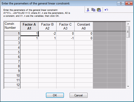
Next, specify the factor constraints. Click the Specify the additional constraints button, and enter the constraints as follows:

As described in the Introductory Overview, you specify the constraints in terms of the weights for the linear equations that have to be greater than/equal to 0 (zero). The weights shown above are direct "translations" of the linear constraints that we want to enter, as defined above. To accept these constraints, click OK.

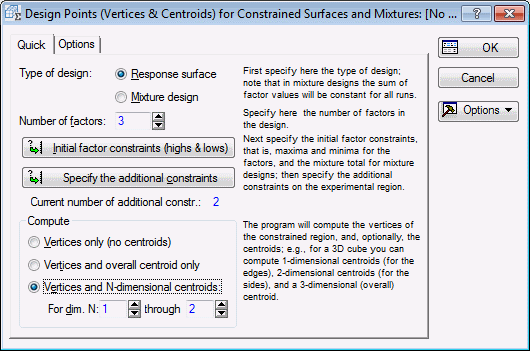
Finally, in the Compute group box, select the Vertices and N-dimensional centroids option button to specify that Statistica also computes the centroids for all two-dimensional sides of the hyperpolyhedron. The dialog box will now look like this.

Now click OK, and Statistica will process the constraints to first compute the vertex points.

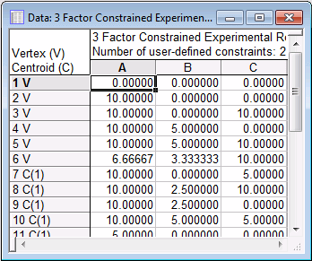
To review the vertex and centroid points, click the Summary: Display design button. A portion of the spreadsheet is shown below in Standard order.

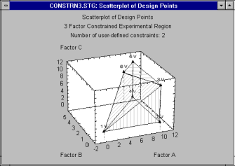
For example, in the results dialog box, click the 3D Scatterplot of points button (note that by default only the vertex points are plotted).

The graph shown above was enhanced to bring out the shape of the constrained region (simply rotate the graph a little to the left, then use the drawing tools to connect the points, and fill the regions facing the observer, to enhance the 3D effect).  

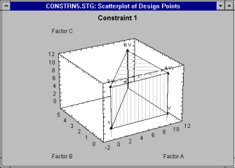
Let us first consider constraint number 1: the values for factor A must be at least twice as large as those for factor B. Clearly, as you move along the horizontal axis for factor A you can see that values for factor B that are valid (inside the sub-region) are always half or less than those for factor A.

For illustration, shown below is the region defined by constraint number 1 alone.

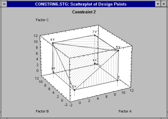
 The consequences of constrained number 2 are also clearly visible (constraint 2 was that values for factor A and B combined must be greater than or equal to those for factor C).

Thus, when factor B is equal to zero, then the constraint simplifies so that the values for C must be less than or equal to those for A; this is clearly reflected in the triangle facing the observer in the A-C plane at xB = 0.

Shown below is the region defined by constraint number 2 alone.

Now, in your mind, put the two constraints together and it is easy to see how the 3D cone-shaped region shown first is the intersection of the two constraint regions shown above.

y = a + b1*x1 + b2*x2 +b3*x3

   +b11*x12 + b22*x22 + b33*x32

   +b12 *x1*x2 + b13 *x1*x3 +b23*x2*x3

These types of models are discussed in the Introductory Overview. On the Confounding tab, select the Lin./quad main effects + 2-ways option button. Then click the Correlation matrix button.

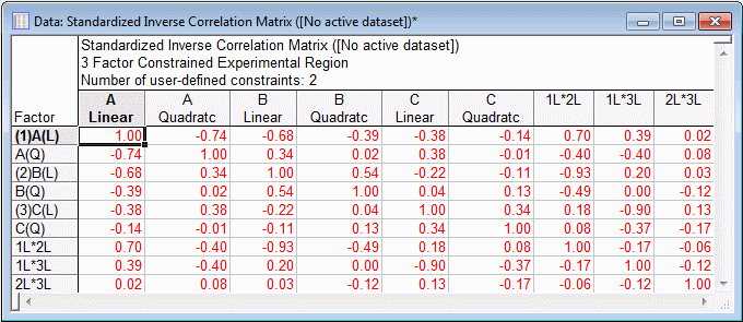
These are the correlations for the factor effects computed from the coded factors for all points (vertices and centroids). To see the inverse of this correlation matrix, return to the results dialog box, and click the Inverse button.

Shown above is the Standardized Inverse of the design matrix (which is the second spreadsheet that will be produced). This matrix can be interpreted as the correlation matrix of the parameter estimates, once we have collected the data. Thus, the entries in this matrix tell you how redundant the effect estimates are, and, in turn, how efficient the design is in extracting information from the experimental region of interest.

This example will be continued in Example 10.2, where we will use the optimal design facilities and try to improve on this simple design consisting of all vertex and centroid points.

See also, Experimental Design.