Naive Bayes Classifier Introductory Overview
The Naive Bayes Classifier technique is based on the so-called Bayesian theorem and is particularly suited when the dimensionality of the inputs is high. Despite its simplicity, Naive Bayes can often outperform more sophisticated classification methods.

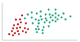
To demonstrate the concept of Naïve Bayes Classification, consider the example displayed in the illustration above. As indicated, the objects can be classified as either GREEN or RED. Our task is to classify new cases as they arrive, i.e., decide to which class label they belong, based on the currently exiting objects.
Since there are twice as many GREEN objects as RED, it is reasonable to believe that a new case (which hasn't been observed yet) is twice as likely to have membership GREEN rather than RED. In the Bayesian analysis, this belief is known as the prior probability. Prior probabilities are based on previous experience, in this case the percentage of GREEN and RED objects, and often used to predict outcomes before they actually happen.
Thus, we can write:

Since there is a total of 60 objects, 40 of which are GREEN and 20 RED, our prior probabilities for class membership are:


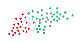
Having formulated our prior probability, we are now ready to classify a new object (WHITE circle). Since the objects are well clustered, it is reasonable to assume that the more GREEN (or RED) objects in the vicinity of X, the more likely that the new cases belong to that particular color. To measure this likelihood, we draw a circle around X which encompasses a number (to be chosen a priori) of points irrespective of their class labels. Then we calculate the number of points in the circle belonging to each class label. From this we calculate the likelihood:

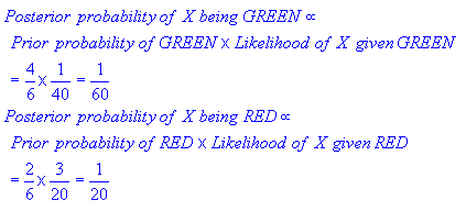
From the illustration above, it is clear that Likelihood of X given GREEN is smaller than Likelihood of X given RED, since the circle encompasses 1 GREEN object and 3 RED ones. Thus:
Although the prior probabilities indicate that X may belong to GREEN (given that there are twice as many GREEN compared to RED) the likelihood indicates otherwise; that the class membership of X is RED (given that there are more RED objects in the vicinity of X than GREEN). In the Bayesian analysis, the final classification is produced by combining both sources of information, i.e., the prior and the likelihood, to form a posterior probability using the so-called Bayes' rule (named after Rev. Thomas Bayes 1702-1761).

Finally, we classify X as RED since its class membership achieves the largest posterior probability.
Note. The above probabilities are not normalized. However, this does not affect the classification outcome since their normalizing constants are the same.
Technical Notes
In the previous section, we provided an intuitive example for understanding classification using Naive Bayes. In this section are further details of the technical issues involved. STATISTICA Naive Bayes classifiers can handle an arbitrary number of independent variables whether continuous or categorical. Given a set of variables, X = {x1,x2,x...,xd}, we want to construct the posterior probability for the event Cj among a set of possible outcomes C = {c1,c2,c...,cd}. In a more familiar language, X is the predictors and C is the set of categorical levels present in the dependent variable. Using Bayes' rule:
where p(Cj | x1,x2,x...,xd) is the posterior probability of class membership, i.e., the probability that X belongs to Cj. Since Naive Bayes assumes that the conditional probabilities of the independent variables are statistically independent we can decompose the likelihood to a product of terms:
and rewrite the posterior as:
Using Bayes' rule above, we label a new case X with a class level Cj that achieves the highest posterior probability.
Although the assumption that the predictor (independent) variables are independent is not always accurate, it does simplify the classification task dramatically, since it allows the class conditional densities p(xk | Cj) to be calculated separately for each variable, i.e., it reduces a multidimensional task to a number of one-dimensional ones. In effect, Naive Bayes reduces a high-dimensional density estimation task to a one-dimensional kernel density estimation. Furthermore, the assumption does not seem to greatly affect the posterior probabilities, especially in regions near decision boundaries, thus, leaving the classification task unaffected.
STATISTICA Naive Bayes provides several choices for modeling to suit your analysis. These include normal, lognormal, gamma and Poisson density functions:

Note. Poisson variables are regarded as continuous since they are ordinal rather than truly categorical. For categorical variables, a discrete probability is used with values of the categorical level being proportional to their conditional frequency in the training data.
