Example 1: Power and Sample Size Calculation for the Independent Sample t-Test
Selecting an analysis type
In this example, we will perform power calculations for the Independent Sample t-Test.
Ribbon bar. Select the Statistics tab. In the Advanced/Multivariate group, click Power Analysis to display the Power Analysis and Interval Estimation Startup Panel.
Classic menus. From the Statistics menu, select Power Analysis to display the Power Analysis and Interval Estimation Startup Panel.
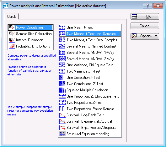
The analysis types are displayed in the left pane of the Startup Panel. There are four basic types of analyses: Power Calculation, Sample Size Calculation, Interval Estimation, and Probability Distributions. The right pane lists the kinds of analysis situations for which the Power Analysis module provides customized analysis.
Ensure that Power Calculation is selected, and then double-click Two Means, t-Test, Ind. Samples to display the Independent Sample t-Test: Power Calc. Parameters dialog box. This kind of dialog box, in which you enter the fixed parameters for the analysis, is the first to appear in all the power calculations.
Selecting baseline parameters
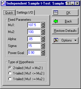
On the Power Calculation parameters Quick tabs (in this case the Independent Sample t-Test: Power Calc. Parameters - Quick tab), you enter the fixed, or baseline, parameters for the analysis in the fields in the Fixed Parameters group box.
The Independent Sample t-Test is one of the classic tests in statistics. In the two-tailed version of the test, the null hypothesis H0 is tested against the alternative H1, where
μ1 is the population mean for Group 1, and μ2 is the population mean for Group 2. The Two-Sample t-Test assumes that the two populations compared have normal distributions, and that the standard deviations are the same in the two populations. To analyze power for a particular situation, you enter the baseline parameters for the situation in this dialog box.
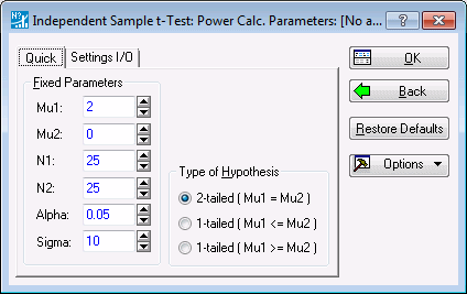
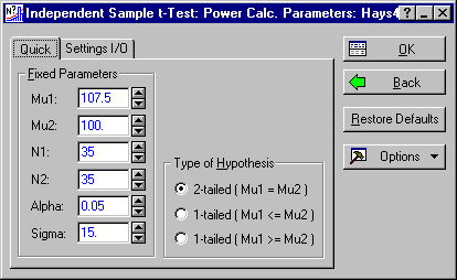
Suppose, for example, you are in the planning stages of an experiment in which you intend to compare two groups on a characteristic where the population standard deviation is 15 in both groups. Subjects are reasonably expensive and difficult to obtain in your line of research, and you anticipate running the study with 25 subjects in each group.
Group 2, the control group in the study, can be (reasonably) assumed to have a population mean of 100. Ascertaining the mean for Group 1, the experimental group, is of course the whole purpose for running the experiment, but you would be disappointed if the treatment were not effective enough to elevate the Group 1 mean to 107.5. Assume that the test is performed with a Type I error rate of a = .05.
Enter the above numbers into the fields on the Quick tab as shown below.
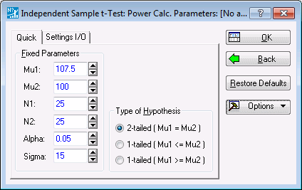
Click the OK button to move to the next stage of the analysis.
Calculating power
The Independent Sample t-Test: Power Calc. Results dialog box is used to investigate power for the situation specified in the Independent Sample t-test: Power Calc. parameters dialog box.
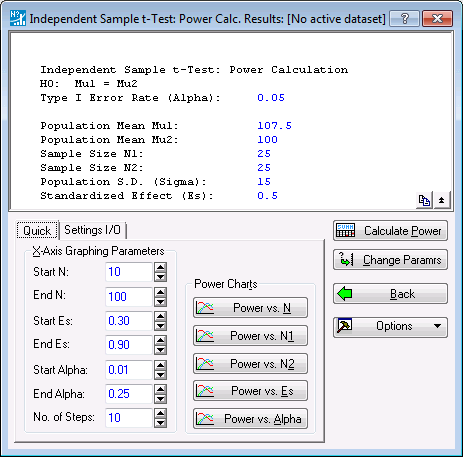
The summary box at the top of the dialog box shows the baseline parameters that have been established for the analysis. In addition to the baseline parameters, Statistica also shows the Standardized Effect (Es) corresponding to the values of m1, m2, and σ.
Es, calculated in this case as:
is the difference between the two means in standard deviation units.
Baseline parameters can be altered at any time by returning to the Power Calculation parameters dialog box (in this case, Independent Sample t-Test: Power Calc.). There are two ways of returning to the previous dialog box. Click the Back button in the Results dialog box, or press the Esc key to return to the preceding dialog box without recording changes to the X-Axis Graphing Parameters on the Power Calculation parameters Quick tab. Click the Change Params button to return to the preceding dialog box and save any changes to the X-Axis Graphing Parameters that have been entered.
To calculate statistical power for the baseline parameters currently in effect, click the Calculate Power button. A spreadsheet containing the result of the power calculation is produced.

The spreadsheet reports Power as .4101 for this combination of parameters.
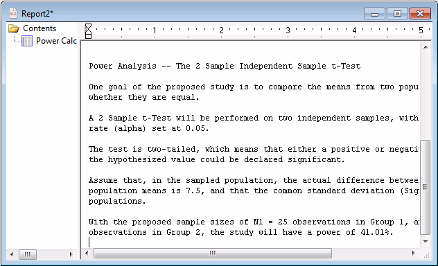
For the convenience of the user who must report power calculations (e.g., in a journal article or grant proposal), the results of the analysis can also be presented in protocol paragraph form in a report, from which they can be copied to the Clipboard.
The protocol paragraph will be sent to a report only if the appropriate settings are selected in the Analysis/Graph Output Manager. To display this dialog box, click the Options button in the Results dialog box, and select Output. From the Report Output drop-down list, select either Multiple Reports (one for each Analysis/Graph) or Single Report (common for all Analyses/Graphs). From the Supplementary detail drop-down list, select Comprehensive.
Clearly, in this case, the power is inadequate. To analyze why, we first digress briefly. Above, we discussed the notion of a Standardized Effect (Es). To understand the full importance of this notion, reflect briefly on the artificiality of the example as we have presented it so far. We have imagined a situation in which the experimenter, to calculate power, considers, in advance, a particular effect (i.e., the difference μ1 - μ2 between the means of the two conditions), and imagines that he/she somehow knows, in advance, the value of σ, the population standard deviation. In most cases, it is no more likely that the experimenter would know σ than it is that the experimenter would know μ1 or μ2. In other words, power calculation based on the notion that the experimenter might somehow know σ is a convenient but completely artificial notion based on a misguided reading of the examples found in textbooks. Such examples frequently gain credibility by using situations where σ might be known to a reasonable degree of accuracy. Many examples use IQ scores, which are assumed to have a standard deviation of 15, because that is the way they are normed. In fact, you need not know σ, μ1, or μ2 in order to calculate power. Instead, you simply specify the hypothesized experimental effect as a standardized effect, which converts μ1, μ2, and σ into a single number, Es. Es has a number of advantages, one of the most significant being that it is invariant under linear scale changes. So, for example, a standardized effect calculated for height in inches would remain the same if height were rescaled into centimeters. Writers on power analysis have established a number of conventions regarding the meaning of Es. For example, Cohen (1983), in his classic text Statistical Power Analysis for the Behavioral Sciences, suggests the following conventions:
This implies that you don't actually have to know μ1, μ2, and σ to perform power analysis. It in turn implies that, in this case, the standardized effect corresponds to a medium effect size. This suggests that sample size is too small to reliably detect a medium-sized effect in this situation. To investigate how large a sample size might be required to achieve a reasonable level of power, you have several options, which we explore in the next section.
Graphical analysis of statistical power
Since power of .4101, achieved with sample sizes of 25 in each group, is clearly inadequate, you must determine how to attain adequate power in order to make the experiment worth pursuing. One step is to examine the relationship between power and sample size, to see just how bad the situation is.
On the Independent Sample t-Test: Power Calc. Results - Quick tab, in the Power Charts group box, click the Power vs. N button to produce a plot of power versus sample size.
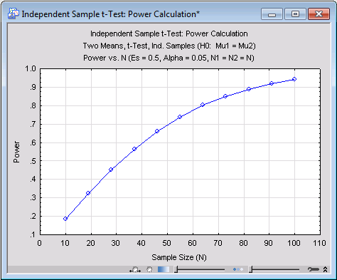
The chart demonstrates that, in order to attain power of .80 (often considered the minimum acceptable level), the sample size must be 64 per group. To boost power to approximately .90, sample size must be increased to approximately 86.
This is a rather disappointing result, given the fact that the Type I error rate is already set at .05, which is in many areas of research the maximum value that journal editors and reviewers will tolerate. The relationship between power and Type I Error rate (a) can be examined by clicking the Power vs. Alpha button to produce the following plot.
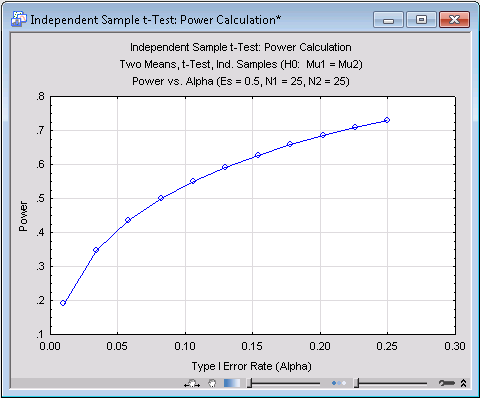
The graph demonstrates the well-known result that power increases as a increases. In this case, even a substantial change in a will not be sufficient, by itself, to boost power to an acceptable level.
For a medium sized effect, sample size must be more than doubled to achieve a respectable level of power. How sensitive is this state of affairs to the size of the standardized effect? Click the Power vs. Es button to produce a plot of power versus standardized effect.

In this case, we can see that power is quite sensitive to the size of the experimental effect in this analysis. Specifically, if the standardized experimental effect is "large" (.80), according to Cohen's (1983) arbitrary standard, then power will be around .78.
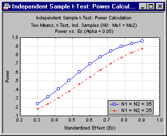
Producing several such graphs can often help you to gain a broader understanding of the interplay between effect size, sample size, and power. Now, click the Change Parameters button to return to the Independent Sample t-Test: Power Calc. Parameters dialog box, and adjust the sample size (N1, N2) upward to 35 for each group. (Remember, if you right-click the microscroll control, the sample size will increment or decrement by 10 units.)
Click the OK button to return to the Independent Sample t-test: Power Calc. Results dialog box. On the Quick tab, click the Power vs. Es button again to generate a graph of power vs. standardized effect size for a sample size of 35 per group.
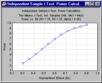
The situation has improved, but not that much. Merging the graphs (via the Graph Data Editor) and adding legends (via the Plots Legend command selected from the Insert menu) gives an even clearer picture. For medium-to-large effects, a sample size increase of 10 per group increases power by .10 to .15.
- Calculating Sample Size
- In the preceding section, we studied the relationship between power, sample size, and the size of an experimental effect by plotting power as a function of these variables. By plotting power against sample size, and observing where the graph intersected with a value of .80, we could see that, with a "medium effect" corresponding to Es = .50, a sample size of approximately 64 was needed to achieve a power of .80.
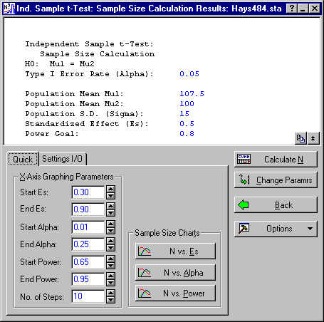
An alternative, more direct approach, is to allow the Power Analysis module to perform the calculation. Click the Back button in the Results dialog box to return to the Independent Sample t-Test: Power Calc. Parameters dialog box. Then click the Back button again to return to the Startup Panel. From the Startup Panel, select Sample Size Calculation as the analysis type and Two Means, t-Test, Ind. Samples as the analysis situation.
Click the OK button to display the Independent Sample t-Test: Sample Size Parameters dialog box, which is used to enter the baseline parameters for sample size calculations. If you have switched to this dialog box after analyzing power for the Independent Sample t-Test, the parameters that are common to the two dialog boxes will be retained.
On the Quick tab, adjust the Power Goal to .80, then click the OK button to display the Ind. Sample t-Test: Sample Size Results dialog box.
Baseline parameters are shown in the summary box at the top of the dialog box. To calculate the N per group needed to achieve power at least equal to the Power Goal, click the Calculate N button.
The resulting spreadsheet contains the original baseline parameters, the Required N (per group), and the Actual Power for Required N. This value will be greater than or equal to the Power Goal, because sample size is an integer value, and it is seldom possible to have an actual power, for a given N, that is exactly equal to the Power Goal. Some power analysis software programs report power for a particular N as being equal to the Power Goal. Often the two values will be very close. However, it is easy to demonstrate situations where the Actual Power for Required N is substantially greater than the Power Goal, and in that case such programs report a value that is substantially in error.
Note also that Statistica automatically writes a "protocol" describing the results of the analysis to the report window if the appropriate settings are selected in the Analysis/Graph Output Manager (described previously in this example).
In this case, Statistica verifies what we saw earlier in the graph of power versus sample size: an N of 64 per group is required to produce power greater than .80.
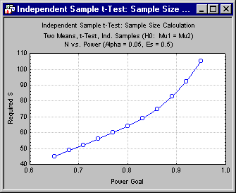
- Graphical Analysis of Sample Size
- To understand how effect size (Es), Type I error rate (a), and the Power Goal affect required sample size, it is often productive to plot graphs relating these quantities. Click the N vs. Power button on the
Quick tab to see how the required sample size varies as a function of required power.
The graph demonstrates how, as the Power Goal increases from the "acceptable" level of .80 toward higher values, the Required S (sample size N) increases. The graph is positively accelerated, which means that the cost of a power increase at the lower levels is less than the cost at higher levels. Click the N vs. Es button to show the effect of standardized effect size on required sample size. As one would expect, larger effects require a smaller sample size to detect at a given level of power.
Notice also the steep rise in Required Sample Size when the effect moves from the "medium" value of .5 toward the "small" value of .2. Clearly, very large values of N are required to detect small effects reliably in the 2-sample t-test.
See also, Power Analysis - Index.