Independent Component Analysis Example
To demonstrate the use of Statistica Independent Component Analysis, we will consider a step-by-step example involving a simple synthetic data set containing two sets of variables (variables 3 and 4) formed by mixing two sets of independent and non-Gaussian signals (variables 1 and 2). We first create and save an ICA model using the Fast ICA algorithm, and then save the model in PMML format, and re-load the file for deployment.
Procedure
-
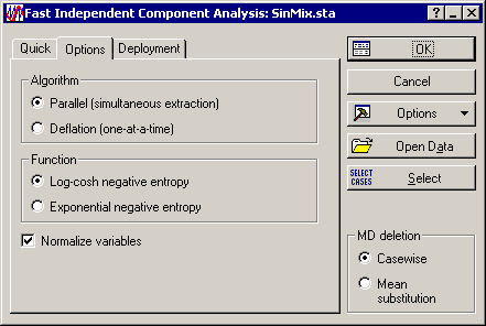
Other settings you may want to change, if and when necessary, are the value of the Alpha parameter of the log-cosh function, used for measuring nongaussianity of the signals, and Tolerance (convergence). The value of the Alpha parameter is restricted to
 .
.
- Further settings of the ICA model can be accessed on the Options tab. Here you can select the method for implementing the Fast ICA algorithm, either Parallel or Deflation. Other settings include the choice of the function used in the measure of nongaussianity (Log-cosh negative entropy or Exponential negative entropy). One option that is recommended to select is the Normalize variables check box. This will specify a form of preprocessing that ensures that all variables are treated on an equal scale and, thus, none of them can bias the analysis merely because of scale or magnitude.
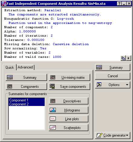
- After you have completed specifying the options for the ICA model, click the OK button to proceed with building the model. This will initiate the Fast ICA algorithm and then display the Fast Independent Component Analysis Results dialog, where you can conclude the analysis.
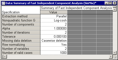
- The Summary box at the top of the Results dialog displays the settings and specifications of the ICA model you just created. Click the Summary button to print the displayed information to a spreadsheet.
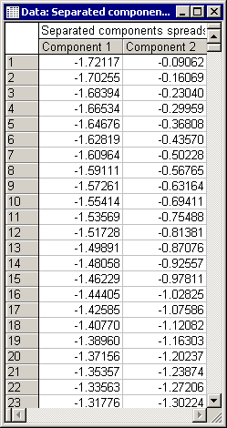
- One of the most important output spreadsheets provided by the ICA model is the estimate of the principal components. Click the Components button to access this information and create the spreadsheet which displays the estimated value of the principal components for each valid case in the data set.
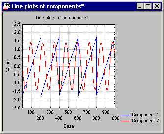
- Alternatively, you may want to view these components in various graph formats. To this end, select (highlight) Component 1 and Component 2 displayed in the Summaries for components list. Click the Line plots button to display the graph of each component against case number in one graph window.
-
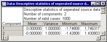
To further analyze the principal components, you may want to print their descriptive statistics (mean, variance, minimum, and maximum). To achieve this click the Descriptives button.
Advanced users may also produce further results using the options on the Advanced tab. These options and their definitions are further discussed in the Statistica Electronic Help and the topic.
Note: The ICA model displayed in the Results dialog is not permanent. This means that clicking the Cancel button will result in the loss of the model you have created. To create a permanent record of your results, use the Code generator option to save the current model in a programming language of your choice. These include C/C++, Visual Basic and PMML. The C/C++ format is particularly suitable for deploying models outside the Statistica environment. If you want to deploy your ICA models via the Statistica Independent Component Analysis, you must use the PMML language. You can access this option from the Code generator drop down menu; select PMML script to display a standard Statistica Report containing the deployment code in PMML language. Copy and paste the entire content of this file into a notepad, and then save it under a name and folder of your choice for later use.

Using ICA for Deployment
You can use your saved ICA models for deployment whenever needed. To do this, you first need to have a data set loaded in the Statistica environment. This data set need not be the same as the one you used to create the model, i.e., training data. In fact, this data set is often different from the training data.
Procedure
- Select the Deployment of existing models check box on the Deployment tab of the Startup Panel. Now, you have the choice of selecting your analysis variables manually by clicking the Variables button, or via the Variable selection via PMML option.
- Click the Load models button to display a file selection dialog. Locate and select a PMML file you have saved.
- Then, run the deployed model. As before, clicking the Components button will create a spreadsheet displaying the principal components as estimated by the deployed ICA model given the new (deployment) data set. The Line plots, Scatterplots, and Histogram options will display the same information in the respective graph formats.