Example 10: Confidence Intervals and Special Tests on the Multiple Correlation
The exact distribution of the squared multiple correlation coefficient is difficult to compute. Consequently, a number of power analysis books and programs rely on approximations that, while generally reasonably accurate, can result in non-negligible errors under some conditions (Gatsonis & Sampson, 1989). STATISTICA Power Analysis calculates the exact distribution of the squared multiple correlation under the assumption that the observed variables have a multivariate normal distribution.
In this example, we examine a number of power analysis, sample size computation, interval estimation, and hypothesis-testing procedures that can be performed with the STATISTICA Power Analysis module.
- Confidence Intervals on the Coefficient of Determination
- The coefficient of determination, R2, is reported routinely as a byproduct of a multiple regression analysis. Along with the sample R2 value, a significance level for the test of the 1-tailed hypothesis
against the alternative
H1: P2 > 0
is usually provided. (P2 is the population equivalent of R2.) These values frequently are not very informative, because (a) the estimate of the coefficient of determination is often subject to substantial sampling error, and (b) the "nil" hypothesis that the coefficient of determination is zero is often completely unrealistic.
A confidence interval on P2 is a much more effective way to present the information that has been obtained from the sample than simply quoting a point estimate and a significance level. For one thing, the standard hypothesis test can be performed with the confidence interval, because the hypothesis test will reject at the α significance level if and only if the 1 - 2α confidence interval fails to include zero. Moreover, the width of the confidence interval provides a valuable indication of the precision of estimation obtained from the analysis.
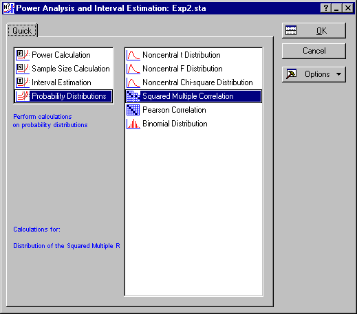
To perform the confidence interval estimation, select Power Analysis from the Statistics menu to display the Power Analysis and Interval Estimation Startup Panel. From the Startup Panel, select Interval Estimation and Squared Multiple Correlation.
Click the OK button to display the Multiple R2: Interval Estimation dialog.
Now suppose that you had just completed a multiple regression analysis in which there were 15 predictor variables, and a sample size of N = 104. The observed sample value for R2 is reported as .30.
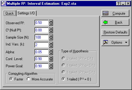
To analyze these values, enter 0.30 in the Observed R2 box, 104 in the Sample Size (N) box, 15 in the number of Ind. Vars (k) box, 0.05 in the Alpha box, and 0.90 in the Conf. Level box. Make sure that the 1-tailed (P2 = 0) option button is selected under Type of Hypothesis. The dialog should look like this:
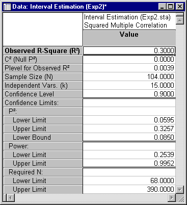
Now click the Compute button. STATISTICA displays a spreadsheet with the results of calculations.
First, note that STATISTICA reports a probability level for the observed R2 of .0039. The observed value of 0.30 is significant beyond the .01 level. The confidence interval for P2, however, demonstrates that the population coefficient of determination has not been measured with a high degree of precision. The 90% confidence interval ranges from .0595 to .3257. The program also reports a 90% lower bound, or 1-tailed confidence interval. This suggests that you can be 90% confident that the population coefficient of determination is no less than .085. This demonstrates that although the observed R2 is statistically significant, there is not strong evidence that the proportion of variance accounted for by the predictor variables is substantial.
STATISTICA also reports post hoc confidence intervals on statistical power. In this case, the confidence interval on power is quite wide, ranging from .2539 to .9952. This is not surprising because power is directly related to the size of the population squared multiple correlation, and the confidence interval on that quantity is quite wide. What this means is that the result we just observed is consistent with the notion that power was quite low, or quite high.
The confidence interval on P2 can also be converted into a confidence interval on the sample size needed to achieve the current power goal. This interval says that we can be 90% confident that the sample size needed to achieve a power of .90 in this study is between 68 and 390. So the sample size actually employed (104) may be about 50% too large, or may be, in the long run, way too small.
These confidence intervals dramatize that statistical significance need not translate into usable levels of precision of estimation.
- Testing a Hypothesis of Minimal Correlation
- In many applications, the hypothesis of zero multiple correlation is not a particularly interesting hypothesis to test, because it is almost certainly false. A more interesting hypothesis to test might be that the coefficient of determination is less than or equal to a target value (representing some minimal acceptable level of variance accounted for by the regression). For example, Murphy and Myors (1998) suggest testing minimal effect values like .01 or .05. In this section, we demonstrate how to
- Find critical values for testing any hypothesis about the squared multiple correlation;
- Find a probability level for an observed value of R2;
- Assess power for testing such a hypothesis against a specified alternative that P2 = .30;
- Calculate required sample size for a particular power goal, when testing a hypothesis of "minimal effect."
Suppose, for example, we wanted to test the null hypothesis that P2 ≤ .05 against the alternative that P2 > .05, in a situation where there are 10 predictor variables, the sample size is 200, and the significance level is .01. To obtain the critical value of R2 for the test, simply use the probability distribution calculator.
Go back to the Startup Panel (by pressing the ESC key) and select Probability Distributions and Squared Multiple Correlation.
Click the OK button to display the Multiple R2 Probability Calculator dialog.
This is a 1-tailed test, so our critical value will have a cumulative probability of .99 in order for α to be .01. Enter .05 in the P2 box, 10 in the Ind. Vars. (k) box, 200 in the Sample Size (N) box, and 0.99 in the Cum. p box. Select the R2 option button under Compute to specify the Observed R2 as the quantity to compute. Finally, click the Compute button to obtain the critical value. The dialog box should look like this:
We have determined the critical value to be .1915626.
Determining the cumulative probability, or the "p-value," is easy in this dialog. To calculate the 1-tailed significance level, ensure that (a) the (1 - Cumulative p) check box is selected, and that the 1 - p option button is selected under Compute. Enter the Observed R2 for which you want to compute the significance level. For example, suppose you observe a sample R2 value of .205, and want to know the significance level. Enter .205 in the Observed R2 box, and click the Compute button. The dialog should appear as below:
To compute power in this situation when the true coefficient of determination is .30, display the Multiple R2 Power Calculation Parameters dialog. Click the Back button to return to the Startup Panel, and select Power Calculation and Squared Multiple Correlation.
Click the OK button to display the Multiple R2 Power Calculation Parameters dialog. Enter the actual value of P2 as .30, 0.05 as the C2(Null P2), 10 as the Ind. Vars. (k), 200 as the N, and 0.01 as the Alpha. Also, be sure to select the appropriate 1-tailed hypothesis by selecting the 1-tailed (P2 <= C2) option button under Type of Hypothesis. The dialog should look like this when you are ready to compute:
Click the OK button to display the Multiple R2 Power Calculation Results dialog.
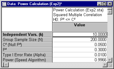
To calculate power of this test of minimal effect, click the Calculate Power button. This will display a spreadsheet with the results of the power calculation.
In this case, we see that the power is quite high, perhaps higher than we need. Money and time might be saved by reducing the sample size. This raises the question, "How big a sample size would we need to have power of .90 in this situation?"
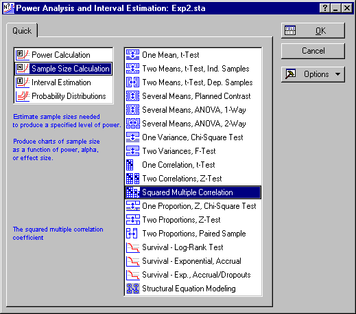
To perform this calculation, go back to the Startup Panel (by pressing the ESC key twice), and select Sample Size Calculation and Squared Multiple Correlation.
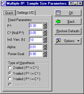
Click the OK button to display the Multiple R2 Sample Size Parameters dialog.
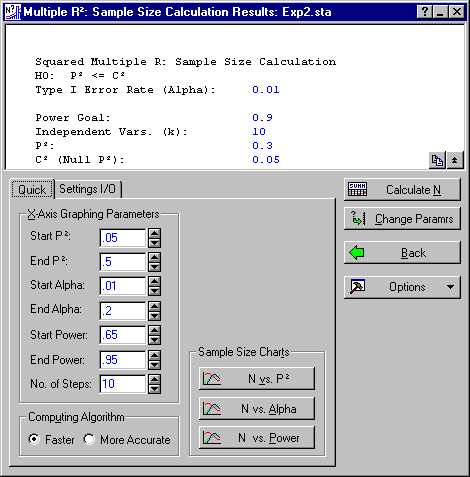
As you can see, the parameters are already correct for performing the desired calculation. Click the OK button to display the Multiple R2 Sample Size Calculation Results dialog.
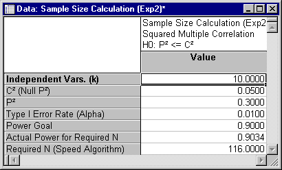
Click the Calculate N button to calculate the required sample size.
It turns out that a sample size of 116 would be adequate to produce power of .90 in this situation.
See also, Power Analysis - Index.


