Example 1: Actuarial Life Table
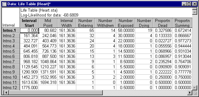
In this example, you compute a life (survival) table for these data, estimate the survival, probability, and hazard functions for different time intervals, and see which theoretical distribution best fits the survival function. See Survival Analysis Examples - Overview and Data File for a description of the data file used in this example.
Specifying the Analysis
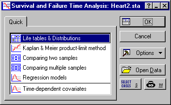
- Select Survival Analysis from the Statistics - Advanced Linear/Nonlinear Models menu to display the Survival and Failure Time Analysis Startup Panel.
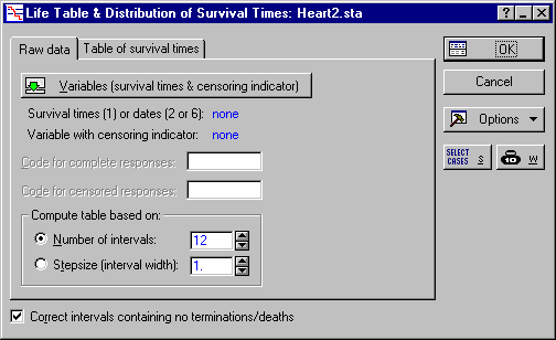
- Ddouble-click Life tables & Distributions to display the Life Table & Distribution of Survival Times dialog box.
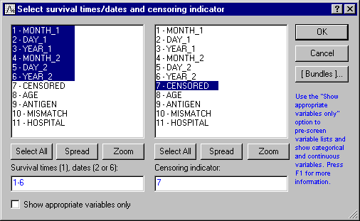
- The Survival Analysis module automatically understands dates as well as any other measurements of survival times. If you click the Variables button and select 6 variables, then Statistica interprets the first three variables as the month, day, and year, respectively, marking the beginning of the respective observation, and the subsequent three variables as the month, day, and year, marking the termination of the observation (due to failure or censoring).
- Cclick the Variables button to display the standard variable selection dialog box. Here, select the first 6 variables as the Survival times (1), dates (2 or 6). As explained above, Statistica interprets the first and fourth variable in the list as months, the second and fifth as days, and the third and sixth as years. Next, specify variable Censored as the Censoring indicator variable in the variable selection dialog box.
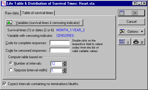
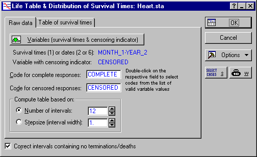
- Click OK to return to the Life Table & Distribution of Survival Times dialog box, which now looks like this.
- Double-click in the Code for complete responses field to display the Variable 7 dialog box. Here, select Complete and click OK. In the same manner, double-click Code for censored responses field and select Censored.
- In addition, you can specify the Number of intervals for the life table, or the Stepsize (interval width). You can also specify whether the intervals in which there are no deaths/terminations are adjusted so that survival distributions can be fitted by selecting the Correct intervals containing no terminations/deaths check box when fitting survival distributions, and clearing this check box when generating a life table for descriptive purposes only.
Reading an Aggregated Life Table
Note that instead of raw data, the Survival Analysis module also accepts already tabulated survival times as input (select the Table of survival times tab).
Specifically, a file with tabulated data should contain 3 variables with the following information:
- The lower limits for each time interval,
- The number of individuals withdrawn alive from each interval, and
- The number of individuals dying in each interval.
This is not the case in the Heart.sta data file, so return to the Raw data tab.
Fitting a Theoretical Survival Distribution
Goodness of fit
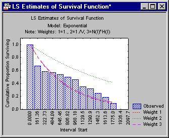
The logic of this goodness of fit Chi-square test is described in the Introductory Overview. In short, the test is based on the comparison of the likelihood of the respective model with the null model; that is, the model that allows for separate hazard estimates in each interval. If this test is significant, you can conclude that the fitted distribution is significantly different from the observed data, and therefore, you reject it as a model for the survival times. In the previous illustration, none of the different parameter estimates for the exponential distribution seems to fit the observed survival distribution.
Choosing a distribution
You can review the parameter estimates for the different distributions by first selecting the distribution from the Results for model box and then clicking the Parameter estimates button on the Quick tab. If you review all of the distributions, you can find that the only one yielding a non-significant fit is the Weibull distribution with weighted least squares parameter estimates.
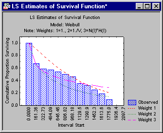
Shown below is a plot of the survival function with the expected values under the Weibull distribution indicated as lines in the plot. (Click the Plot of survival function button on the Function plots tab.)
It appears that the third set of parameters (Weight 3) provides a reasonable fit to the data; the Chi-square test for that model is not significant (p=.56). Therefore, you can conclude that the Weibull distribution with the third set of parameters provides a good theoretical model for the data.
Hazard and probability density function
The Introductory Overview describes the computation of the hazard rate and probability density function. In short, the hazard rate is an estimate of the probability (per time unit) that an observation that has not failed prior to a particular interval, fails in that interval; the probability density function is an estimate of the probability density of failure per time unit in the respective interval.
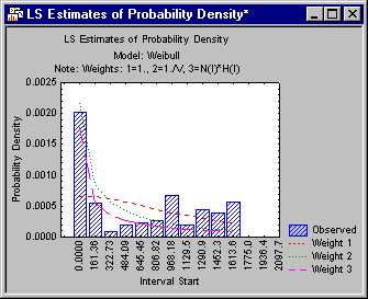
In order to evaluate the goodness of fit of the chosen theoretical distribution, you can also review these functions in plots, together with the values for the observed distribution (click the Plot of hazard function and Plot of probability density function buttons on the Function plots tab). Usually, the hazard rate increases over time, because the probability of failure generally increases as time progresses.
The probability density usually decreases over time, reflecting the fact that, overall, the probability (density) of failure is greater in the earlier time intervals.

