Example 9: Using Contingency Tables to Compute Chi-Square Tests for Independence

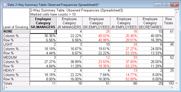
A contingency table summarizes the frequencies across two variables. For example, it may be interesting to compare variables such as Level of Smoking and Employee Category. Does a difference in smoking rate exist across various employee categories? The data may list the employees, their job titles, and level of smoking. This data can then be tabulated into a contingency table, showing the frequencies across the levels of these variables as shown in the table below.

At times, the data are collected in a contingency table format. Instead of each employee listed in a spreadsheet, the summarized contingency table is all that is available. When this is the case, and additional statistics are required such as chi-square tests for independence or row and column percentages, the data require rearrangement. This topic focuses on a statistical analysis when starting with a contingency table.

Rearranging the Data for Analysis

Statistica performs complex data analysis procedures, and therefore has structural requirements about the data used for analysis. Data are not always collected in a format that is ready for analysis in Statistica. Data preparation tools are available in Statistica to ease the transition between the original data and data for analysis in Statistica. These data preparation tools include Stacking and Unstacking, Recode, Transpose, and spreadsheet formulas. For this example, the Stacking and Unstacking tool will be used.

The example data set, Smoking.sta, located in the STATISTICA examples folder, is a contingency table showing the crosstabulation frequencies of Level of Smoking: NONE, LIGHT, MEDIUM, and HEAVY, and Employee Category: SR. MANAGERS, JR. MANAGERS, SR. EMPLOYEES, JR. EMPLOYEES, and SECRETARIES. This is summarized data, not raw data. Statistica requires raw data for analysis. This data can easily be transformed to raw data with a few steps, and then the data can be analyzed.

1. Open the Smoking.sta data file. On the ribbon bar, select the Home tab. In the File group, click the Open arrow and select Open Examples to display the Open a Statistica Data File dialog box. Double-click the Datasets folder, and then open the data set. This spreadsheet is the contingency table.

2. Select the Data tab. In the Transformations group, click Stack to display the Unstacking/Stacking dialog box. Select the Stacking tab, and click the Variables button. In the variable selection dialog box, select all four variables and click the OK button.

In the Unstacking/Stacking dialog box, in the Destination variable name field, type in Frequency. In the Code variable name field, type in Level of Smoking.

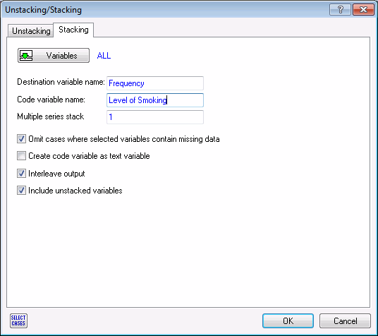
Click OK. A new spreadsheet is created with two variables, Frequency and Level of Smoking.

3. On the ribbon bar, select the Data tab. In the Variables group, click the Variables arrow and from the drop-down list, select Add to display the Add Variables dialog box. In the How many field, enter 1. In the After field, enter 2. In the Name field, enter Employee Category.

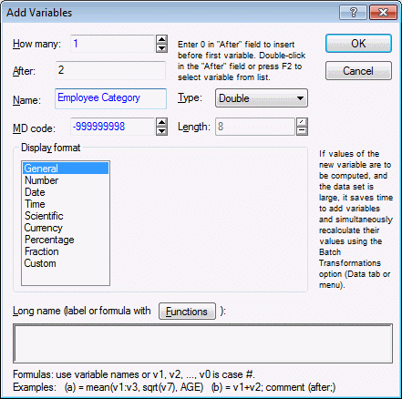
Click OK.  A new variable is added to the spreadsheet.

4. On the ribbon bar, select the Data tab. In the Cases group, click Names to display the Case Names Manager dialog box. In the Transfer case names group box, select the To option button. Double-click in the Variable field to display the Select Variable dialog box. Select Employee Category and click OK.

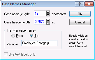
Click OK in the Case Names Manager dialog box to update the Employee Category variable with the case names.

5. On the ribbon bar, select the Tools tab. Click Weight to display the Spreadsheet Case Weights dialog box. In the Status group box, select the On option button. In the Weight variable field, enter Frequency.  

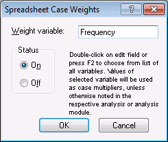
Click OK. If the Setting Spreadsheet Case Weights dialog box is displayed (which further explains the use of case weights), click OK.

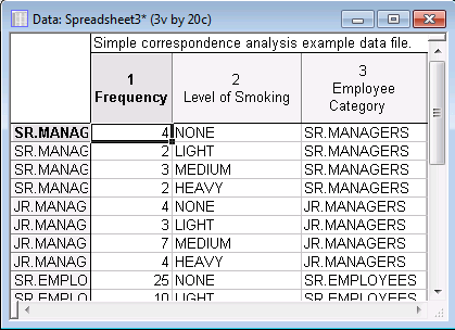
The spreadsheet (shown partially below) is now ready for analysis with the Crosstabulation tool. It contains the two variables for analysis, Level of Smoking and Employee Category. The third variable, Frequency, contains the frequency weights that will be used in analysis.

Analyzing the Data  

The Crosstabulation tool can be used for creating contingency tables as well as for the calculation of several statistics including various independence tests and percentages of rows, columns, and total. Now that raw data has been created from the original contingency table, the data can be analyzed in Statistica.

1. On the ribbon bar, select the Statistics tab. In the Base group, click Basic Statistics to display the Basic Statistics and Tables Startup Panel. Select Tables and banners and click OK to display the Crosstabulation Tables dialog box.

2. On the Crosstabulation tab, click the Specify tables (select variables) button to display the Select up to 6 lists of grouping variables dialog box. In List 1, select Level of Smoking. In List 2, select Employee Category. Click OK in the Select up to 6 lists of grouping variables dialog box, and click OK in the Crosstabulation Tables dialog box to display the Crosstabulation Tables Results dialog box.

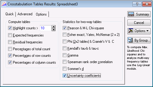
3. Select the Options tab. In the Compute tables group box, select the Percentages of row counts check box and the Percentages of column counts check box. In the Statistics for two-way tables group box, select the Pearson & M-L Chi-square check box.

4. Select the Advanced tab. Click the Detailed two-way tables button to create the two-way table output and chi-square output.

The 2-Way Summary Table output gives the contingency table along with the requested row and column percents. The first Column %, 36.36%, is interpreted as follows: of senior managers, 36.36% report that they are non-smokers. The first Row %, 6.56%, is interpreted as: of non-smokers, 6.56% were senior managers. This table is helpful in showing trends between the two variables.

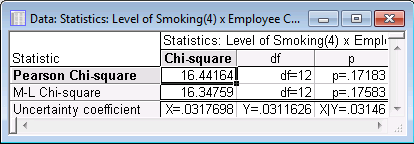
The second output data file contains the independence test statistics. The test is evaluating the independence of Level of Smoking and Employee Category. If the two are independent, no significant relationship exists between them. If the null hypothesis is rejected and the variables are found to be dependent, it can be concluded that Level of Smoking varies across Employee Category. At this point, the relationship could be further explored with row, column, and total percentages.

The Chi-square test is 16.44164 with an insignificant p-value of 0.1783. This indicates that the two variables are independent or that no significant relationship exists between Level of Smoking and Employee Category.