Response Optimization Example - Regression
| Parameter | Description |
|---|---|
| Crime Rate | Per capita crime rate by town |
| Residential Land Zone | Proportion of residential land zoned for lots over 25,000 sq.ft. |
| Non-retail Business acres | Proportion of non-retail business acres per town |
| Charles River | Charles river dummy variable (1 if tract bounds river; 0 otherwise) |
| Nitric Oxide | Nitric oxide concentration - parts per 10 million |
| Average Rooms | Average number of rooms per dwelling |
| Owner Occupied Units | Proportion of owner occupied units built prior to 1940 |
| Distance to Employment | Weighted distances to five Boston employment centers |
| Accessibility to Highways | Index of accessibility to radical highways |
| Property Tax Rate | Full value property tax rate per $10,000 |
| Pupil-Teacher Ratio | Pupil-Teacher ratio by town |
| % of Lower Status | % of the lower status of the population |
| Value of occupied homes | Median value of owner occupied-homes in $1,000s |
Number of cases = 506
Several neural network models were trained for predicting the observed house prices in this data set, and the models were saved in PMML format. Our task is to use these models to apply a Response Optimization analysis to house prices in the Boston area.
Procedure
-
To display this spreadsheet, click the
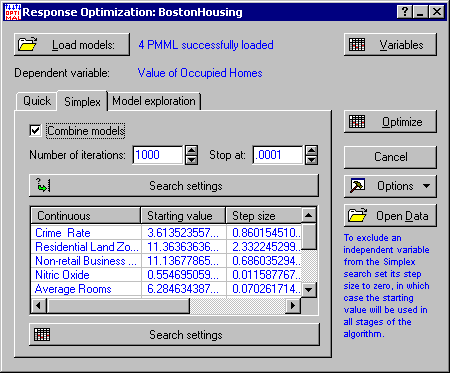
Variables button in the Response Optimization Startup Panel.
This information helps you to select sensible option settings for your analysis. For example, the minimum and maximum of the variables can help you with the settings of the Simplex, Grid, and Random algorithms (see the documentation for the Search settings button on the Simplex, Grid, and Random tabs). By setting the minimum and the maximum of the Simplex algorithm, for instance, equal to the minimum and the maximum of the appropriate variables in the data set, you can in fact confine the Simplex search to regions of the independent space that was included in the original data set. This confinement is important since optimization may lead to unreliable results should it be conducted outside regions falling way off from the boundaries of the original data set.
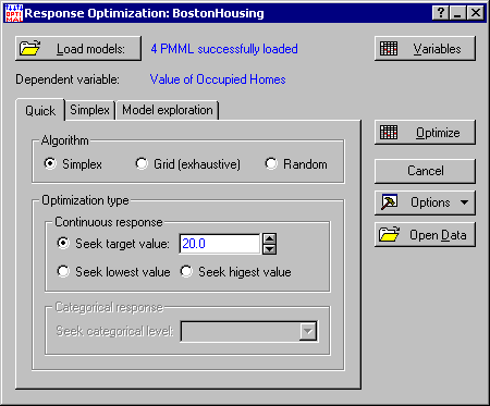
- Going back to the real estate scenario described previously, our task now is to find what kind of house our customer can get given a fixed budget. Let's assume that the budget is $20K. This means we have to set the value of the Seek target value option (in the Optimization type group box of the Quick tab) to 20.
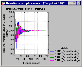
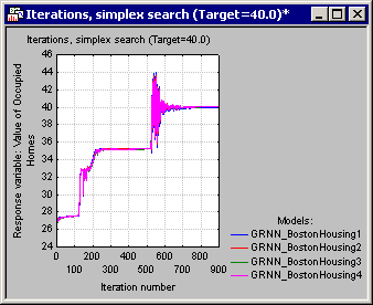
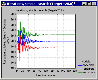
- Next, click the Optimize button in the Startup Panel to initiate the Simplex algorithm. While the algorithm is in progress, a progress bar is displayed showing the predictive model undergoing optimization and the iteration number. When the search is complete, output in the form of spreadsheets and a graph is displayed, the last of which is the plot of model predictions (y-axis) against iteration number (x-axis).
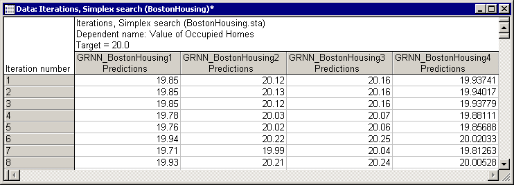
- By reviewing this graph (which contains one plot per model) you can tell if the algorithm has succeeded in finding the desired value and how many iterations it took to converge. Note that the same information displayed in this graph can also be viewed in the form of a spreadsheet (Iterations, Simplex search spreadsheet).
-
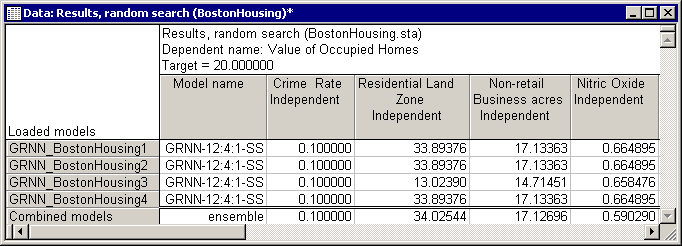
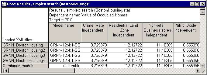
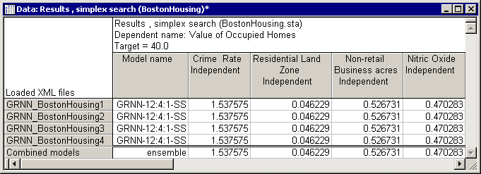
The Results spreadsheet is perhaps the most important output.
Here you can view the final solutions found by the algorithm for each predictive model, i.e., the set of independent values (house attributes) for which the predictive models yielded the desired response (desired house price). This is mainly a "finite data size" effect, i.e., having a limited number of cases in the training data set. However, since data sets are always finite in size, such variations among predictive models may always exist. To alleviate this problem, we need to combine the existing predictive models (should there be more than one). Models combined to cooperate on making predictions are called ensembles, which are known to have a better generalization ability (i.e., to predict unseen data more accurately).
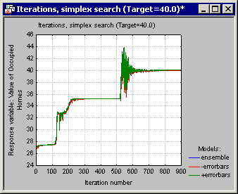
With Statistica Response Optimization, you can form ensembles out of existing models by selecting the Combine models check box on the Simplex tab. This functionality enables you to form ensembles out of the existing models.
-
So, instead of making house price predictions based on one model, let's combine our models. To do so, select the
Combine models check box and click the
Optimize button once again.
When the search is complete a number of spreadsheets and graphs are displayed. One particularly useful bit of information is the variance displayed by the ensemble. A large value should be a cause for concern since it is an indication that the predictive models yielded substantially different response values given the same set of independent values. Note that the agreement among the ensemble members can also be viewed from the iterations plot of the ensemble. This information is conveniently displayed as errorbars.
- You can repeat the same optimization for any house price the customer is willing to pay. In our next search we can, for example, double the price by setting the Seek target value option to 40, and then observe what kind of improvement the target property might have over those sold for a mere $20K.
- A glance at the results spreadsheets for houses priced at $20K and $40K shows significant improvements in many property attributes such as Crime Rate and Average Rooms.
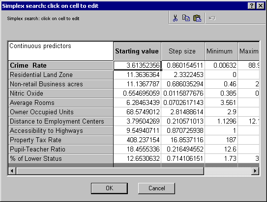
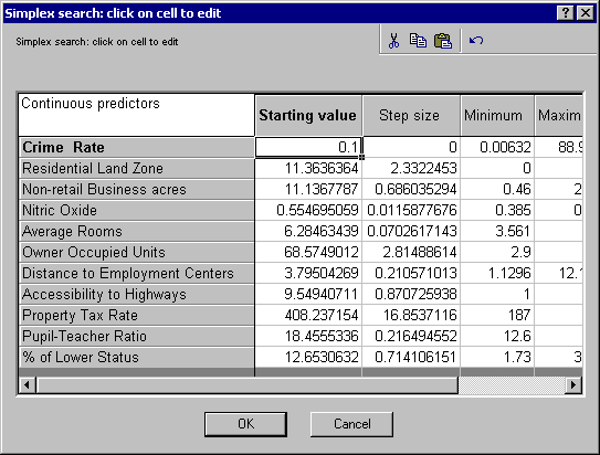
- Finally, let's assume that the customer has strong preferences toward living in an area where the crime rate is low while he or she is still willing to pay only $20K. Thus, we want to find what kind of housing one can purchase given the price and subject to the condition Crime Rate = %0.1. To do this, select the Simplex tab and click the Search settings button to display a standard Statistica general user entry spreadsheet.
- On the spreadsheet, locate the Crime Rate entry and change both the Starting value and Step size to 0.1 and 0, respectively.
- Click the OK button to make your modifications permanent.
- On the Quick tab, change the value specified in the Seek target value option back to 20. Next, click the Optimize button once again, and compare the results with the previous ones.


Correcting Simplex Failure
The Simplex technique is a guided optimization algorithm that can find the desired solution in a finite number of steps.
However, just as any other algorithm, it may sometimes fail to find the desired solution. In cases such as this, you can use the Grid or Random algorithms as alternatives. These algorithms are implementations of simple techniques based on brute computing power. In this section, we use the Random algorithm to search for houses in the Boston area. For the application of the Grid algorithm to optimization tasks see the step-by-step example for classification.
As before, we want to find the attributes of a $20K property located in an area with a crime rate of 0.1%, this time using the Random algorithm.
Procedure
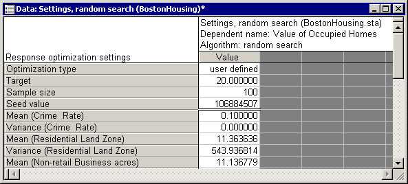
- Select the Random option button on the Response Optimization Startup Panel Quick tab. As before, set the house price, using the Seek target value option, to 20.
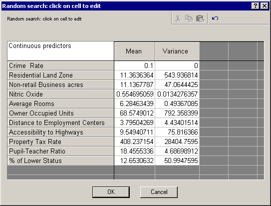
- To fix the Crime rate at 0.1, set the mean for the sampling distribution of this variable to 0.1 and its variance to 0.
- Also, make sure that the Sample size is set to a suitable value on the Random tab. The larger the variances for the sampling distributions the more samples you need in order to produce accurate results.
- Next, click the Optimize button. When random sampling is complete, two spreadsheets are displayed showing the settings of the Random algorithm and the search results.