Example 3: Sample Size Calculation in Factor Analysis
Choosing a sample size in common factor analysis is complicated by the facts that (1) until recently, there was no firm statistical basis for forming such a judgment, and (2) there are a number of different significance tests that can be performed in factor analysis, many of which have differing power characteristics. Statistica Power Analysis provides, in its Structural Equation Modeling power analysis module, facilities that can be used for estimating power and sample size requirements in a number of different situations, including ordinary exploratory factor analysis (see Factor Analysis), confirmatory factor analysis (see Structural Equation Modeling (SEPATH), and causal modeling. In this example, we will examine how to perform some basic power and sample size calculations in exploratory factor analysis.
The basic rationale for performing convenient power and sample size calculations in structural equation modeling contexts was introduced by MacCallum, Browne, and Sugawara (1996).
Specifying baseline parameters
Ribbon bar. Select the Statistics tab. In the Advanced/Multivariate group, click Power Analysis to display the Power Analysis and Interval Estimation Startup Panel.
Classic menus. From the Statistics menu, select Power Analysis to display the Power Analysis and Interval Estimation Startup Panel.
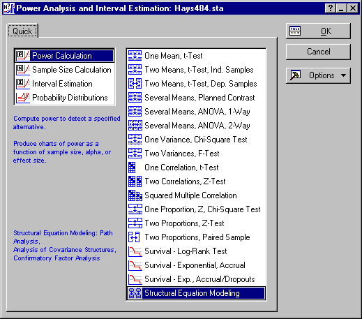
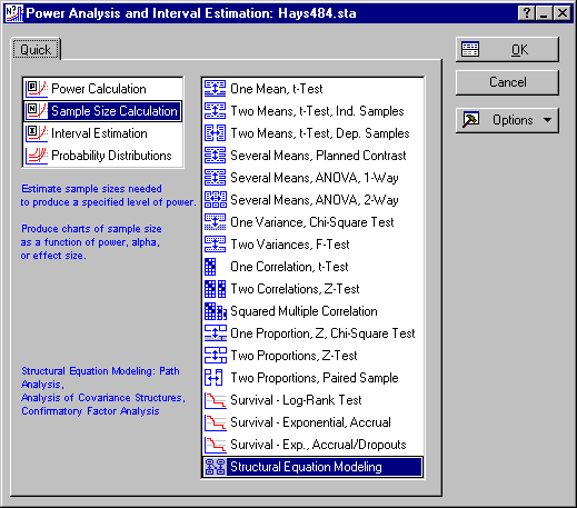
From the Startup Panel, select Sample Size Calculation and Structural Equation Modeling.
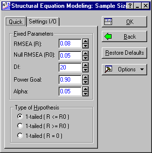
Click the OK button to display the Structural Equation Modeling: Sample Size Calculation Parameters dialog box.
Suppose you were planning to perform an exploratory factor analysis, using the method of maximum likelihood, as implemented in the Statistica Factor Analysis module with 10 observed variables and wished to assure power of at least .80 to detect departures from reasonable goodness of fit. MacCallum, Browne and Sugawara (1996) suggest performing a test of the hypothesis that the RMSSE is less than or equal to .05, versus the alternative that the RMSSE is greater than .05. In their article, they examine sample size required to attain a power of .80.
A key decision in any exploratory factor analysis is to decide on the number of common factors to retain. This decision is a complicated one, and clearly involves interplay between substantive and statistical considerations. The traditional approach, implemented in many computer programs, is to begin by fitting a single common factor to the data, and perform a chi-square test of the hypothesis that the model fits perfectly. If this hypothesis is rejected (at, say, the .05 level), then the number of common factors is increased to two, and the process is repeated. This continues until the hypothesis test fails to reject.
Numerous authors have criticized this sequential chi-square testing approach. One criticism is that the hypothesis being tested is unrealistic and unnecessarily stringent. The hypothesis of perfect fit of a complex model is almost invariably false, and it makes no sense to test it. Moreover, since the testing strategy is Accept-Support, (see Sampling theory and hypothesis testing logic), the experimenter who wants to find a small number of factors is rewarded, in a sense, for running an experiment with low power.
One solution to this problem is to test a more reasonable hypothesis, i.e., that fit is good though not perfect, and guarantee reasonable power to detect departures from this hypothesis.
Suppose that the experimenter plans to start with a single common factor, and fit models with increasing numbers of factors until the hypothesis that the Root Mean Square Error of Approximation (RMSEA) is less than or equal to .05 cannot be rejected. The question, is, how large a sample size would be required to assure a power of at least .80 when the population RMSEA is at least .08, for each of these tests?
Exploratory factor analysis with p observed variables and m factors produces a chi-square statistic with degrees of freedom equal to
df = [(p - m)2 - (p + m)] / 2
Using this equation, we can determine degrees of freedom for various values of m, the number of common factors. For example, with p = 10, and m = 1, degrees of freedom are
[(10 - 1)2 - (10 + 1)] / 2 = 35
With p = 10, and m = 2, degrees of freedom are
[(10 - 2)2 - (10 + 2)] / 2 = 26
In like manner, we can construct a table for degrees of freedom corresponding to 3, 4, and 5 common factors. We obtain
The table shows that we may need to run as many as five separate factor analyses on the same data, before settling on an appropriate m. We would like to determine a sample size that will guarantee a power of .80 for all of these tests.
- Calculating Required Sample Size for Tests of Near Fit
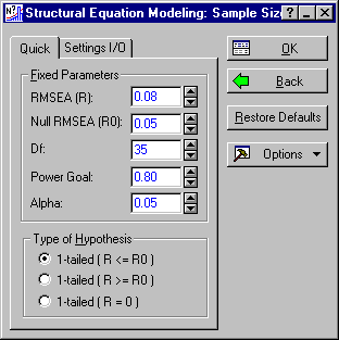
- To perform the calculations, we use the guidelines suggested by MacCallum, Browne, and Sugawara (1996). On the
Structural Equation Modeling: Sample Size Parameters - Quick tab, enter 35 in the degrees of freedom (Df) box and 0.80 in the Power Goal box.
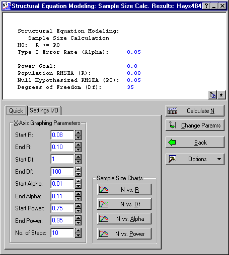
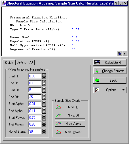
Click the OK button to display the Structural Equation Modeling: Sample Size Calc. Results dialog box.
To calculate N for the current parameters, click the Calculate N button. A spreadsheet with the results of the calculation is then displayed.
In this case, it appears that the ability to distinguish reliably between good fit and somewhat mediocre fit will require a sample size of 279.
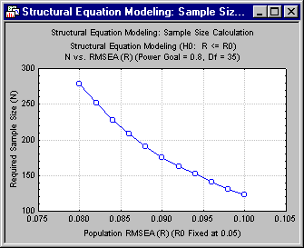
Note: this judgment is subject to many qualifications. For one thing, at this stage we have no idea how sensitive our sample size estimate is to minor variations in the specifications of the calculation. For example, suppose our designation of .08 for "mediocre fit" is somewhat stringent. If we were to relax the requirement somewhat, and require power of .80 to detect an RMSEA of .10, what effect would this have on required N?Statistica makes it very easy to conduct this sensitivity analysis. First, we examine required N as a function of the RMSEA value. The default values of the X-Axis Graphing Parameters on the Structural Equation Modeling: Sample Size Calc. Results - Quick tab will analyze the effect of the value of RMSEA from .06 to .11 (see the Start R and End R boxes). Click the N vs. R button to examine the relationship.
Note how the power curve changes character dramatically as R varies below .08. Detecting an R of .07 will be almost twice as expensive as detecting an R of .08. On the other hand, the power curve becomes substantially flatter for RMSEA values above .08. Let's zoom in on the relationship by varying the range of the graph from .08 to .10. Adjust the parameter range (Start R and End R) in the X-Axis Graphing Parameters group.
Then click the N vs. R button again to redraw the graph. In this range, the relationship between required N and RMSEA is much more linear.
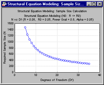
Recall that there are five potential tests, corresponding to 35, 26, 18, 11, and 5 degrees of freedom. We can examine the N required for all these simply by setting the appropriate graphics parameters. Enter 5 in the Start Df box, 35 in the End Df box, and 30 in the No. of Steps box.
Then click the N vs. Df button to create the graph.
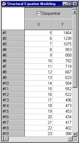
The graph includes values of the required N for all the df values we are interested in. To create a table of these values, select Graph Data Editor from the View menu.
Using these values, we can quickly augment our previous table with the required N values. Note that, as the number of factors increases (and the number of degrees of freedom decreases), the required sample size increases substantially.
Here is the revised table.
When testing for a single common factor with 35 degrees of freedom, a sample size of 279 is adequate. When testing the adequacy of a 5-factor model with five degrees of freedom, a sample size of 1464 is required. What is particularly discouraging about the implications of the table is that the trend relating required N to number of factors (m) runs in exactly the opposite direction that we would prefer. In general, we would expect the actual RMSEA to be higher with smaller m, and consequently it may well be that the required N for lower values of m is unnecessarily pessimistic.
This chart also suggests that, with the sample sizes traditionally employed, statistical tests will not be able to distinguish reliably between RMSEA values of .05 and .08 when the number of factors is large, relative to the number of variables.
In an important practical sense, the problem is not quite as severe as it seems. Remembering that our goal is to select an appropriate number of factors, and that, traditionally, factor analysts insist on a number of factors for which degrees of freedom are positive. Hence, the key decisions occur for values less than 5, because once a number of factors equal to 5 is achieved, the significance test becomes somewhat less important. At that point, the largest number of factors has been achieved, and the question becomes more one of estimating the RMSEA with a confidence interval than it does rejecting a hypothesis in order to select an appropriate number of factors.
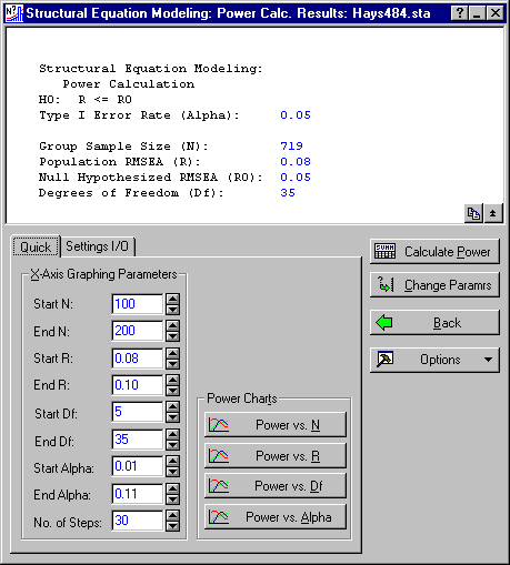
Consequently, a compromise decision would be to use the sample size for m = 4, i.e., 719. This sample size can be expected to generate outstanding power for m = 1,2,3 and power of .80 for m=4. This can be verified by returning to the Startup Panel (by clicking the Back button on both the Structural Equation Modeling: Sample Size Calc. Results and the Structural Equation Modeling: Sample Size Parameters dialog boxes), and selecting Power Calculation and Structural Equation Modeling.
Click the OK button to display the Structural Equation Modeling: Power Calculation Parameters dialog. Enter 719 in the N box, and keep the other parameters as they are.
Click the OK button to display the Structural Equation Modeling: Power Calc. Results dialog box.
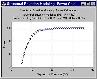
Now, click the Power vs. Df button to examine the power values.
You can see that this compromise leaves the power at only .51 for the m=5 test, although the power is more than adequate for all the other tests. However, the situation is not quite as bad as it seems, because if the actual RMSEA is .09 instead of .08, the power for the m = 5 test rises rather dramatically to .73. Thus, click the Back button on the Structural Equation Modeling: Power Calc. Results dialog to return to the Structural Equation Modeling: Power Calculation Parameters - Quick tab and enter 0.09 in the RMSEA (R) box. Then click the OK button to return to the Results dialog box and click the Power vs. Df button.
In the final analysis, selection of an appropriate sample size for tests of significance in exploratory factor analysis is something of an art, involving a series of careful analyses and compromises. Part of the decision-making process will depend on your prior knowledge of the subject matter, and what the acceptable limits are on the number of factors. Clearly, for example, if you decide a priori that any number of factors above three is completely unacceptable, then you can reduce the sample size for this study to 473, realizing that you will have adequate power for all of the significance tests you plan to do.
- Computing Sample Size for Tests of Perfect Fit
- So far, we have examined power from the perspective advanced by MacCallum, Browne, and Sugawara (1996). From their view, perfect fit, corresponding to an RMSEA of 0, is not a reasonable null hypothesis to be testing in factor analysis. We support this view. However, Statistica
Power Analysis is fully capable of computing power and required sample size for the old-fashioned hypothesis of perfect fit. For example we could test the hypothesis that fit is perfect against the alternative that it is not perfect. In this case, the null and alternative hypotheses would be
Let's re-examine the situation we just examined by computing the required sample sizes to test this hypothesis, when the actual RMSEA corresponds to fair fit, i.e., .08, and the required power is .80.
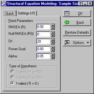
Click the Back button on both the Structural Equation Modeling: Power Calc. Results and the Structural Equation Modeling: Power Calculation Parameters dialog boxes to return to the Startup Panel. Here, select Sample Size Calculation and Structural Equation Modeling and then click the OK button to display the Structural Equation Modeling: Sample Size Parameters dialog box. Enter 0 in the Null RMSEA (R0) box and make sure the Power Goal is .80. Note that the Type of Hypothesis automatically changes to 1-tailed (R = 0).
Click the OK button to display the Structural Equation Modeling: Sample Size Calc. Results dialog box. Enter 5 in the Start Df box, and 35 in the End Df box.
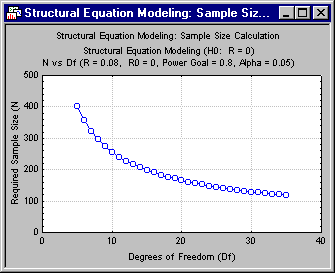
Click the N vs. Df button to generate a plot of required N for degrees of freedom from 5 to 35.
Of course, the ability to distinguish between perfect fit and fair fit requires far smaller sample sizes than the ability to distinguish between good fit and fit that is only fair.
There are considerations other than power in choosing a sample size for a factor analysis. In particular, boundary cases tend to arise when the sample size is too small. After settling on a sample size that yields adequate power, you should test the performance of factor analysis procedures by using the Monte Carlo facilities in Statistica Structural Equation Modeling module. An example of how Monte Carlo investigation can alert you to an inadequate sample size (that will create a high a priori probability of boundary cases) is given in the Statistica Structural Equation Modeling documentation.
See also, Power Analysis - Index.