Distribution Fitting Example
The Distribution Fitting module is used to evaluate the fit of observed data to some theoretical distributions. Refer to Types of Distributions for descriptions of the available distributions. Also note that the Survival Analysis module contains specialized routines for fitting censored (incomplete) survival or failure time data to the Weibull and Gompertz distribution.
The data file used for this example is Irisdat.sta (part of the data file is shown below). This file contains data reported by Fisher (1936) on the lengths and widths of sepals (Sepallen, Sepalwid) and petals (Petallen, Petalwid) for 50 flowers of three types of iris. A discriminant function analysis of this data set is also described in the Discriminant Analysis Example.
The distributions of the four variables describing the lengths and widths of sepals and petals will now be examined. Specifically, it is expected that those measures follow the normal distribution.
Ribbon bar. Select the Home tab. In the File group, click the Open arrow and from the menu, select Open Examples. The Open a STATISTICA Data File dialog box is displayed. Irisdat.sta is located in the Datasets folder. Next, select the Statistics tab. In the Base group, click Distribution Fitting to display the Distribution Fitting Startup Panel
Classic menus. From the File menu, select Open Examples to display the Open a STATISTICA Data File dialog box; Irisdat.sta is located in the Datasets folder. Then, from the Statistics menu, select Distribution Fitting to display the Distribution Fitting Startup Panel.
Select the Continuous Distributions option button, and then double-click on Normal.
In the Fitting Continuous Distributions dialog box, click the Variable button to display the standard variable selection dialog box. Select variable Sepallen, and then click the OK button.
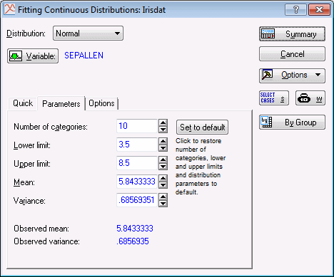
At this point, the data file will be processed and the Parameters tab of the Fitting Continuous Distributions dialog box will show the computed mean and variance as the default values for the Mean and Variance boxes. There are also options on this tab to adjust the Number of categories and the Lower and Upper limits for the computation of the frequency distribution.
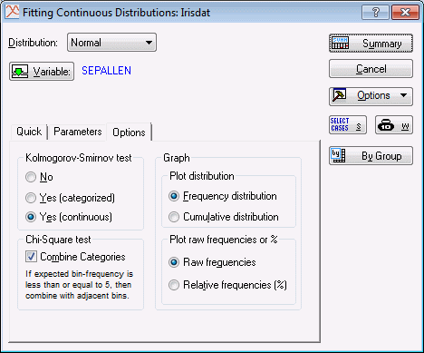
Next, select the Options tab. In the Kolmogorov-Smirnov test group box, select the Yes (continuous) option button. Accept all of the other default selections in this dialog box, and click the Summary button to compute the frequency distribution.
- Test statistics
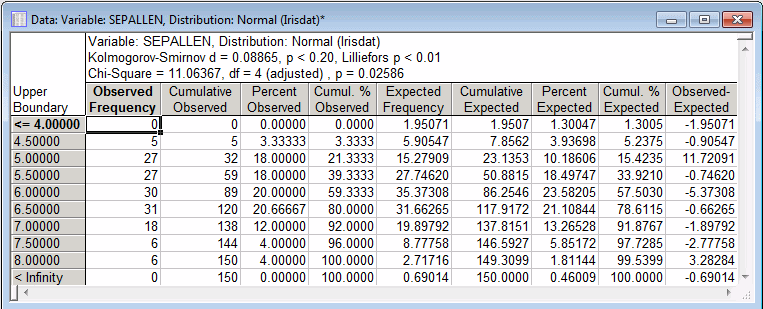
- The Chi-square value is significant at the .05 level (p = .026). Thus, based on the Chi-square test, we would conclude that the distribution deviates significantly from the standard normal distribution. However, the Kolmogorov-Smirnov d test is not significant (p < .20). This pattern of results is not uncommon because the Kolmogorov-Smirnov test is not as much a precise procedure as it is a technique to detect gross deviations from some assumed distribution.
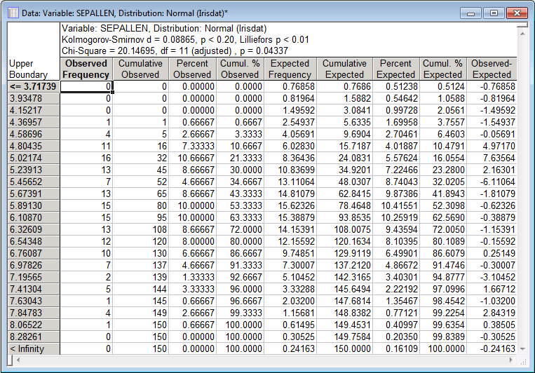
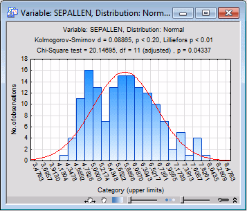
Often, the Chi-square value is greatly affected by the way in which the distribution is "sliced up," that is, by the number of categories and minimum and maximum values that we choose. For example, if we slice the distribution for Sepallen into 23 pieces (enter 23 in the Number of categories box on the Parameters tab), rather than the default 10 categories, the resulting Chi-square value is only marginally significant at the p = .04 level.
Of much greater importance is how the general shape of the observed distribution approximates the hypothesized normal distribution.
Return to the Fitting Continuous Distributions dialog box. On the Options tab, in the Graph group, we can choose to plot a histogram of the Frequency or Cumulative distribution with the Raw or Relative frequencies.
Accept the default graph selections, and on the Quick tab, click the Plot of observed and expected distribution button to produce the frequency histogram for this variable. (Note that you should still have 23 Number of categories on the Parameters tab.)
It seems that the distribution of Sepallen is bimodal, that is, it appears to have two "peaks." Also, a major lack of fit exists on the left side of the observed distribution where the first peak occurs. Thus you would conclude from the analysis that the continuous normal distribution probably does not provide an adequate model for the observed distribution.
See also, Distribution Fitting - Index.


