Example 1: Joining - Tree Clustering
Data File
This example is based on a sample of different automobiles. Specifically, one particular model was randomly chosen from among those offered by the respective manufacturer. The following data for each car were then recorded:
- The approximate price of the car (variable Price),
- The acceleration of the car (0 to 60 in seconds; variable Acceler),
- The braking performance of the car (braking distance from 80 mph to complete standstill; variable Braking),
- An index of road holding capability (variable Handling), and
- The gas-mileage of the car (miles per gallon; variable Mileage)
Scale of Measurement
All clustering algorithms at one point need to assess the distances between clusters or objects, and obviously, when computing distances, you need to decide on a scale. Because the different measures included here used entirely different types of scales (e.g., number of seconds, thousands of dollars, etc.), the data were standardized (via the Standardize command from the Data menu) so that each variable has a mean of 0 and a standard deviation of 1. It is very important that the dimensions (variables in this example) that are used to compute the distances between objects (cars in this example) are of comparable magnitude; otherwise, the analysis will be biased and rely most heavily on the dimension that has the greatest range of values.
- Open the
Cars.sta data file, which contains the standardized data for this example. It is located in the Datasets folder.

- Perform a joining analysis (tree clustering, hierarchical clustering) on this data.
Purpose of Analysis: This is to test whether these automobiles form "natural" clusters that can be labeled in a meaningful manner.
- To display the Clustering Method Startup panel, select Cluster Analysis from the Statistics - Multivariate Exploratory Techniques menu .
- Select Joining (tree clustering) and then click the OK button.
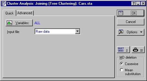
- To display the standard variable selection dialog box and select all of the variables, click the Variables button on the Cluster Analysis: Joining (Tree Clustering) dialog box - Quick tab.
- To return to the
Cluster Analysis: Joining (Tree Clustering) dialog box -
Quick tab, click the
OK button.
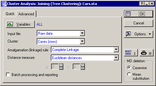
- To cluster the automobile (cases) based on the different performance indices (variables). The default setting of the Cluster box on the Advanced tab is Variables (columns); We need to change this setting. Depending on the research question at hand, one may cluster cases in some instances and variables in others.
- To know whether the cars (cases) form clusters. Select
Cases (rows) in the
Cluster box. Also, select
Complete Linkage in the
Amalgamation (linkage) rule
box.
Distance measures
Remember that the tree clustering method will successively link together objects of increasing dissimilarity or distance. There are various ways to compute distances, and they are explained in the Introductory Overview. The most straightforward way to compute a distance is to consider the k variables as dimensions that make up a k-dimensional space. If there were three variables, then they would form a three-dimensional space. The Euclidean distance in that case would be the same as if we were to measure the distance with a ruler. Accept this default measure (Euclidean distance) in the Distance measure box for this example.
Amalgamation (Linkage) rule
The other issue of some ambiguity in tree clustering is exactly how to determine the distances between clusters. Should we use the closest neighbors in different clusters, the furthest neighbors, or some aggregate measure? As it turns out, all of these methods (and more) have been proposed. The default method (Single Linkage) is the "nearest neighbor" rule. Thus, as we proceed to form larger and larger clusters of less and less similar objects (cars), the distance between any two clusters is determined by the closest objects in those two clusters. Intuitively, it may occur to us that this will likely result in "stringy" clusters, that is, STATISTICA will chain together clusters based on the particular location of single elements. Alternatively, we can use the Complete Linkage rule. In this case, the distance between two clusters is determined by the distance of the furthest neighbors. This will result in more "lumpy" clusters. As it turns out for this data, the single linkage rule does in fact produce rather "stringy" and undistinguished clusters.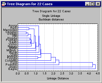
The tree diagram
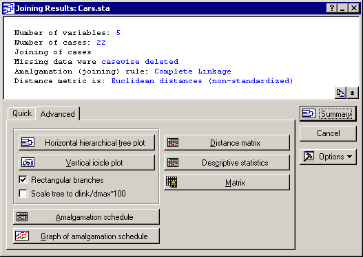
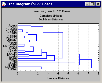
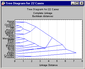
The most important result to consider in a tree clustering analysis is the hierarchical tree. The Cluster Analysis module of STATISTICA offers two types of tree diagrams with two types of branches. For the standard style of tree diagram, select the
Rectangular branches check box and click the
Horizontal hierarchical tree plot button to create a horizontal Tree Diagram (Complete Linkage).
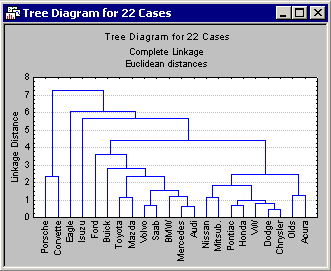
Also, click the
Vertical icicle plot button.
In addition, we can choose to scale the tree plot to a standardized scale with the Scale tree to dlink/dmax*100 check box. Select the
dlink/dmax*100 check box.
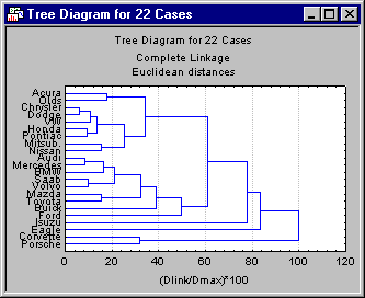
The scale will be based on the previously selected distance measure. Thus, it represents the percentage of the range from the maximum to the minimum distance in the data.
At first, tree diagrams may seem a bit confusing; however, once they are carefully examined, they will be less confusing. The diagram begins on the left in horizontal tree diagrams (or on the bottom in vertical icicle plots) with each car in its own cluster. As we move to the right (or up in vertical icicle plots), cars that are "close together" are joined to form clusters. Each node in the above diagrams represents the joining of two or more clusters; the locations of the nodes on the horizontal (or vertical) axis represent the distances at which the respective clusters were joined.
Identifying Clusters
For this discussion, consider only horizontal hierarchical tree diagrams (see the tree diagram with the standardized scale), and begin at the top of the diagram. Apparently, first there is a cluster consisting of only Acura and Olds; next there is a group (i.e., cluster) of seven cars: Chrysler, Dodge, VW, Honda, Pontiac, Mitsubishi, and Nissan. As it turns out, in this sample the entry level models (more or less) of these brands were chosen. Thus, we may want to call this cluster the "economy sedan" cluster.
A non-graphical presentation of these results is the amalgamation schedule (click the Amalgamation schedule button on the Joining Results dialog box - Advanced tab).
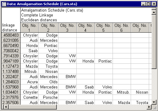
Amalgamation Schedule: The Amalgamation Schedule results spreadsheet lists the objects (cars that are joined together at the respective linkage distances (in the first column of the spreadsheet).
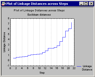
This graph can be very useful by suggesting a cutoff for the tree diagram. Remember that in the tree diagram, as we move to the right (increase the linkage distances), larger and larger clusters are formed of greater and greater within-cluster diversity. If this plot shows a clear plateau, it means that many clusters were formed at essentially the same linkage distance. That distance may be the optimal cut-off when deciding how many clusters to retain (and interpret).