Independent Component Analysis Technical Notes

The Cocktail Party Problem

Imagine being at a party where many people are speaking simultaneously. We are all familiar with how difficult it may be to listen to those we want to hear because of the interfering noise. This is known as the Cocktail Party Problem. The human brain can solve this problem because it has the ability to focus listening attention on a single speaker of choice among a mixture of conversations and background noise. This ability to concentrate on a speaker of choice is known as Blind Source Separation, which attempts, as the name states, to separate a mixture of signals into separate components. The word blind is used to highlight the generally unknown statistical nature of the interfering signals.

One of the most widely used methods for separating mixed signals is known as Independent Component Analysis. This method is central to Statistical Signal Processing with a wide range of applications in many areas of technology including Audio and Image Processing, Biomedical Signal Processing, Telecommunications, and Econometrics. Mixed signals could be emitted by a number of physical objects such as cell phones or brain cells. Irrespective, our task is to decompose the interfering signals into their individual components.

How does ICA work?

Let's consider a case that involves two speakers. We will assume that there are two microphones positioned in different locations recording the speakers' voices. The microphones provide us with two recorded signals in time, which we denote with x₁ and x₂. In ICA, the recorded signals are expressed in terms of the speakers' signals using the representation:

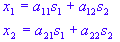
where t denotes time, s₁ and s₂ are the original speakers' signals and the a's are the mixing coefficients, which are dependent on how far the microphones were from the speakers. Using matrix notation, we can re-write the above equation as:

where the mixing matrix is given by:

The task of ICA is to obtain estimates of the original signals s₁ and s₂ (unknown) given the recorded signals x₁ and x₂ (which are known). If we know the mixing coefficients, we can obtain estimates of s₁ and s₂ simply by inverting the linear representation above. Thus:

where A-1 is known as the un-mixing matrix.

In reality, however, the mixing coefficients are unknown. Therefore it is the task of ICA to find estimates of the mixing coefficients before we can extract the signals s₁ and s₂ .

Assumptions

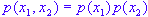
To do so, the ICA method assumes that the original signals are statistically independent. An assumption that may not (and need not) be always true, but one that is vital for finding the principal components s₁ and s₂. Statistical independence means that:

The other assumptions the ICA method uses is that original signals are non-Gaussian and that there are as many as independent signals as the number of recorded signals.

Measure of Nongaussianity

As said before, nongaussianity is one the most important assumptions on which the ICA method is based. In fact we cannot apply ICA without having a measure of nongaussianity. One of the most commonly used measures is known as Negentropy. The entropy of a random variable is the measure of the information that can be obtained by observing that variable. The more unlikely to observe a random variable the more information is gained by observing it. A random variable with a normal distribution has maximum entropy. This means that we can use entropy as a measure of nongaussianity.

Using the entropy concept, Fast ICA uses the following formula for the measure of nongaussianity:

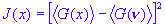
Two popular choice of the non-quadratic G are:

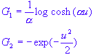
where is a constant.

Pre-processing

ICA algorithms often make use of preprocessing to transform the observed signals to suitable numeric format. The most basic form of pre-processing is Centering, in which the observed signals are centered around their means so that the transformed signals have zero mean:

Another pre-processing technique used by ICA is known as whitening. This technique is applied after centering. It involves linearly transforming the observed signals X into a new set of variables , which are uncorrelated and their variances equal unity:

where T denotes matrix transpose and is the covariance matrix. Using the above, we get the following expression for the whitened variables:

where is the new mixing matrix. is the whitening matrix.

The Fast ICA Algorithm

Fast ICA defines a weight vector w (or a matrix for Parallel extraction, see below). Using the learning rule, this vector is updated such that the projection maximizes the nongaussianity measure . This process is then repeated as many items as needed until a solution is reached

• Choose an initial weight vector w (from random).
• Use the formula to update the weight vector w.
• Normalize the resulting vector using
• Repeat 2 and 3 until the algorithm is converged.

The above steps are a one unit version of the Fast ICA algorithm, known as Deflation, which extracts one principal component at a time. For further details of this method and its multi unit version, known as Parallel or Multiple Extraction, see Aapo Hyvarinen, et al.