Getting Started with Statistica Data Miner
To use the Statistica data mining tools, follow these steps:
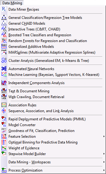
The StatisticaData Mining tab (ribbon bar) and Data Mining menu contain the following options:
- To create a data miner workspace where you can build and maintain complex models
- To select predefined templates of data miner workspaces for simple and complex tasks
- To select Statistica analysis modules for particular specialized analyses
- To guide you through a step-by-step process to simplify the method of predictive model building, use the Data Miner Recipes option
Classic menus
| Option | Description |
|---|---|
| Data Miner - All Procedures | Select this command (located on the Data Mining - Workspaces submenu) to create a new data mining workspace. |
| Data Miner - Data Cleaning and Filtering | Select this command (located on the Data Mining - Workspaces submenu) to choose from a large number nodes for cleaning the data, (for filtering out invalid data values, missing data replacement, user-defined transformations, ranking, standardization). |
| Feature Selection and Variable Screening | You can quickly process very large lists of continuous and categorical predictors for regression and classification problems, and to select a subset that is most strongly related to the dependent (outcome) variables of interest.
The algorithm for selecting those variables is not biased in favor of a single method for subsequent analyses (pick the highest correlations for later analyses using linear models), and the resulting variable lists are made available as mappings into the original data source, so that no actual data need to be copied (such as from a remote data base). |
| Data Miner - General . . . . | Select any of these commands (located on the Data Mining - Workspaces submenu) to display predefined sets of data mining templates for typical types of analysis problems. The General Slicer/Dicer Explorer with Drill-Down command also provides access to a specialized interactive drill-down tool. |
| Neural Networks, Independent Components Analysis, Generalized EM & k-Means Cluster Analysis, Association Rules, General Classification/Regression Tree Models, General CHAID Models, Interactive Trees (C&RT, CHAID), Boosted Tree Classifiers and Regression, Random Forests for Regression and Classification, Generalized Additive Models, MARSplines (Multivariate Adaptive Regression Splines), Machine Learning (Bayesian, Support Vectors, Nearest Neighbors) | These commands display the modules for performing the respective types of analyses interactively, using the standard Statistica user interface. |
| Rapid Deployment of Predictive Models (PMML); Goodness of Fit, Classification, Prediction; Feature Selection and Variable Filtering; Combining Groups (Classes) for Predictive Data-Mining | These commands display the respective specialized modules; Rapid Deployment of Predictive Models quickly generates predictions from one or more previously trained models based on information stored in industry-standard PMML (Predictive Model Markup Language) deployment code. Goodness Of Fit computes various goodness-of-fit statistics and graphs for regression and classification problems. Feature Selection and Variable Screening is used to select variables (columns) from very large data sets or external databases, example, to select subsets of predictors from hundreds of thousands of predictors, or even more than one million predictors. Combining Groups (Classes) for Predictive Data-Mining is used to automatically find and implement a best recoding scheme for the prediction of a continuous or categorical variable from one or more categorical predictors with many classes (example, such as SIC codes with more than 10,000 distinct values). |
2. Select a new data source
Next, specify the input data for the data mining project.
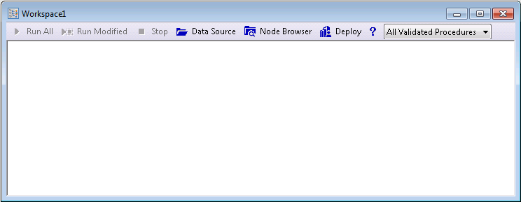
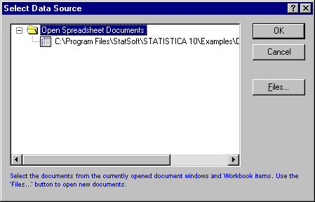
Click the Data Source button on the data miner workspace to display a standard data file selection dialog where you can select either a Statistica data file (Statistica Spreadsheet designated for Input), or a database connection for in-place processing of data in remote databases.
3. Select the variables for the analyses.
Next, select the variables for the analyses.
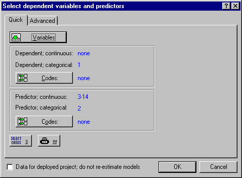
Statistica Data Miner distinguishes between categorical and continuous variables, and dependent and predictor (independent variables).
- Categorical variables are those that contain information about some discrete quantity or characteristic describing the observations in the data file (Gender: Male or Female).
- Continuous variables are measured on some continuous scale (Height, Weight, Cost).
- Dependent variables are the ones we want to predict. They are also sometimes called outcome variables.
- Predictor (independent) variables are those that we want to use for the prediction or classification (of categorical outcomes).
You don't have to select variables into each list. In fact some types of analyses only expect a single list of variables (cluster analysis).
You can also make additional selections, such as specify codes for categorical variables, case selection conditions, or case weights, or you can specify censoring, a learning/testing variable.
Example.
4. Display the Node Browser and select the desired analyses or data management operation.
Next, use one of the following actions:
- Click the Node Browser button on the data miner workspace.
- Display the Node Browser by selecting that command from the Nodes menu
- Press CTRL+B on your keyboard to display the node browser.
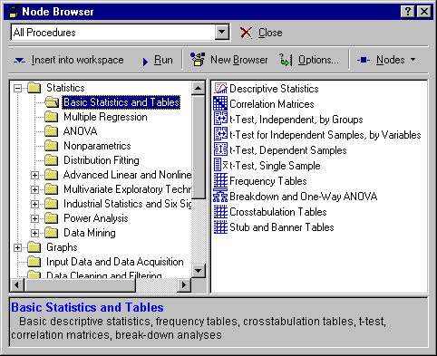
The Node Browser contains all the procedures available for data mining in the data miner workspace. You can choose from more than 260 procedures from for data filtering and cleaning, and for data analysis. By default, all procedures are organized in folders along with the types of analyses that they perform.
However, the Node Browser is fully configurable. You can specify multiple Node Browser configurations, and these customizations are automatically saved along with the data miner workspace. Thus, you can greatly simplify routine analyses by fully customizing the default Node Browser configuration for your work.
- To select analyses (analysis nodes), highlight them in the right pane.
- Click the Insert into workspace button on the Node Browser toolbar. You can also simply double-click on the analysis node of interest to insert it into the workspace. The lower pane of the Node Browser contains a description of the currently highlighted selection.
- Select the nodes for Descriptive Statistics.
- Scroll down in the left pane of the Node Browser.
- Select the folder labeled Classification and Discrimination.
- In the right pane, select
Standard Classification Trees with Deployment.
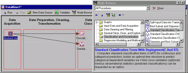
If a data source in the workspace is currently highlighted, it is connected automatically to the nodes as they are selected (inserted) into the workspace.
- You can also use the Connect toolbar button to connect data sources to nodes.
- To delete an arrow, click on it and select Delete from the shortcut menu (displayed by right-clicking your mouse), or press the DEL key on your keyboard.
- You can temporarily disable an arrow by selecting Disable from the shortcut menu. Arrows that are disabled are not updated or recomputed.
5. Run (update) the data miner project.
Next, run the data miner project. All nodes connected to data sources using (non-disabled) arrows are updated, and the respective analyses are produced.
A note on data cleaning, filtering, and EDA
The Statistica Data Miner project workspace is fully integrated into the Statistica data analysis environment. At any point, you can click on a data source or results workbook (spreadsheet, report), either in the Data Acquisition area or in any other area ( data sources created by analyses), to review the respective document.
Also, you can use any of the interactive analyses available in Statistica to further explore those documents (for example, to run simple descriptive statistics or create descriptive graphs to explore the respective results). These types of Exploratory Data Analysis techniques (EDA) are indispensable for data cleaning and verification.
For example, it is useful to always run simple descriptive statistics, computing the minima and maxima for variables in the analyses, to ensure that data errors (impossible values) are corrected before they lead to erroneous conclusions. Also, the various options on the Data menu of the data spreadsheet toolbar are very useful for cleaning and verifying the data in interactive analyses before submitting them to further analyses.
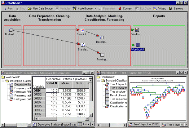
Example.
- Click the Run button.
- Select
Run All Nodes from the
Run menu or press
F5.
Detailed results are created by default for each type of analysis in Statistica Workbooks.
Double-click on a workbook to review its contents. You can also connect all the green arrows to the workbooks into a single workbook, to direct all results to a single container. The complete functionality of Statistica Workbooks is available for these results, so you can perform these actions:
6. Customize analyses, edit results, save results.
The next step is to review the results, edit the analyses, etc.
- In general, click on any icon, and then use the shortcut menu to review the various options available for the object (analysis, data source, output document, result, etc.).
- To review results, double-click on the Workbooks or other documents created by the analyses.
- To direct output to reports instead of workbooks, use the options on the Data Miner tab of the Options dialog box to configure Statistica Data Miner. Example: To edit analyses (change the parameters for the analyses), double-click on the respective analysis icons; this displays the Edit Parameters dialog box, which contains parameters and settings specific to the respective node.
- To edit documents created by analyses for downstream analyses, click on the item, and select View Document from the shortcut menu.
- To delete nodes:
- To save the workspace, select Save from the File menu. The default filename extension for the data miner workspace is .sdm. By default, the program saves all input data sources embedded into the data mining project. Change this default by clearing the Embed input files in Data Miner project files when saving check box on the Data Miner tab of the Options dialog box.
- Example
- To compute various graphical summaries:
- Double click on the Descriptive Statistics node.
- Set the Detail of reported results parameter to All results.
- Click OK.
- Double-click on the Standard Classification Trees with Deployment node.
- Select the V-Fold Cross-validation tab.
- Request V-Fold cross-validation (this is a very important safeguard against over-learning).
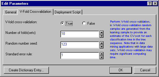
- Click on the General tab.
- Set the Minimum n per node (of the final tree) to 50, which will cause the tree growing procedure to terminate when the node size falls below that number, and to create less complex trees.
- Click the OK button. The two analysis nodes, as well as the workbook nodes, now display with a red frame around them, which denotes that these nodes are not up to date (they are dirty).
- Move the arrow from the Standard Classification Trees with Deployment to point to the same (first) workbook where the descriptive statistics are displayed. To do this, click on the head of the arrow, and drag it over to the first workbook (release the mouse button as your cursor is hovering over the workbook node).
- Delete the now disconnected node (unless you'd like to keep it for reference).
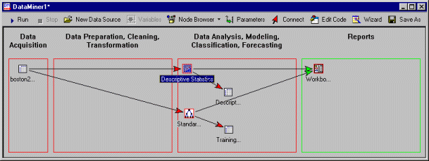
- Next click the
Update button, or press
F5.
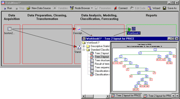
- After all nodes are updated, double click on the (now single) results node to review all results in the workbook. Note that both the Descriptive Statistics as well as the results of the Standard Classification Trees analysis are displayed in the same workbook.
7. Deploy solution (models) for new data.
Statistica Data Miner includes a complete deployment engine for data miner solutions that comprises various tools. For example:
- You can create Visual Basic or C/C++/C# program code in most interactive analysis modules that will compute predictions, predicted classifications, clusters assignments [such as General Regression Models, Generalized Linear Models, General Discriminant Function Analysis, General Classification and Regression Trees (GC&RT), Generalized EM & k-Means Cluster Analysis, etc.]. (See also, Using C/C++/C# Code for Deployment.)
- You can create XML-syntax based PMML files with deployment information in most interactive modules that will compute predictions, predicted classifications, or cluster assignments (the same modules mentioned in the previous paragraph).
- One or more PMML files with deployment information based on trained models can be loaded by the Rapid Deployment of Predictive Models modules to compute predictions or predicted classifications (and related summary statistics) in a single pass through the data; hence this method is extremely fast and efficient for scoring (predicting or classifying) large numbers of new observations.
- General Classification and Regression Trees and General CHAID modules can be used to create SQL query code to retrieve observations classified to particular nodes, or to assign observations to a node ( to write the node assignments back into the database).
- Complex neural networks and neural network ensembles (sets of different neural network architectures producing an average or weighted predicted response or classification) can also be saved in binary form and later applied to new data.
In addition, Statistica Data Miner contains various designated procedures in the (Node Browser) folders Classification and Discrimination, Regression Modeling and Multivariate Exploration, and General Forecaster and Time Series, to perform complex analyses with automatic deployment and cooperative and competitive evaluation of models.
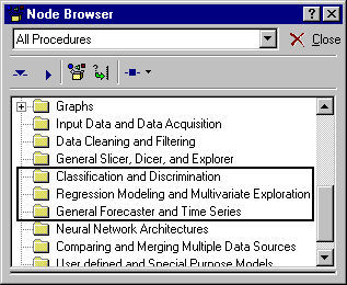
For example, the Classification and Discrimination folder contains nodes for the following:
- Stepwise and best-subset linear discriminant function analysis
- Various tree classification methods
- Generalized linear models procedures
- Different neural network architectures
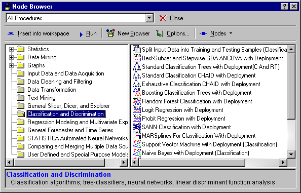
The analysis nodes with automatic deployment are generally named TypeOfAnalysis with Deployment.
Simply connect these nodes to an input data source, update (train) the project, and you are ready for deployment: Connect to the node a data source marked for deployment (select the Data for deployed project check box in the dialog specifying the variables for the analysis), and the program will automatically apply the most current model (tree classifier, neural network architecture) to compute predictions or predicted classifications.
Example
- Start a new data miner project by selecting a predefined project for classification.
- From the
Data Mining - Workspaces – Data Miner - General Classifier (Trees and Clusters) submenu, select
Advanced Comprehensive Classifiers Project.

- Then, click the New Data Source button.
- Select the Boston2.sta data file again.
- Specify Price as the categorical dependent variable.
- Select variable Cat1 as a categorical predictor.
- Select variables ORD1 through ORD12 as continuous predictors.
- Click the Connect button.
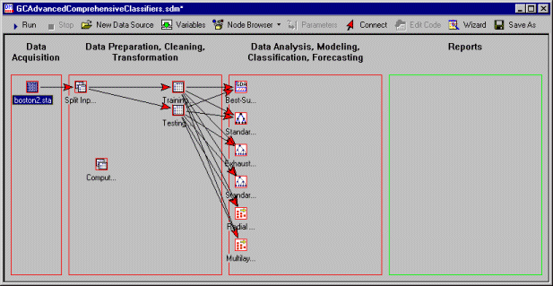
- Connect the data icon to the
Split Input node, which is the main connection point for the
Advanced
Comprehensive Classifiers Project.
-
Now, click the
Run button. A number of very advanced, and somewhat time-consuming, analyses will now be performed:
- The Split Input node in the Data Preparation, Cleaning, Transformation area will randomly select two samples from the input data: One for training the various models for classification, and the other to evaluate the models,(for the observations in the Testing sample) the program will automatically compute predicted classifications and misclassification rates so that the Compute Best Prediction From All Models node (the one that initially is not connected to anything in the Data Preparation, Cleaning, Transformation area) can automatically pick the best classifier, or compute a voted best classification ( apply a meta-learner).
- The program will automatically apply to the Training sample the following classification methods: linear discriminant analysis, standard classification trees (C&RT) analysis, CHAID, Exhaustive CHAID, a radial basis function neural network analysis, and a multiplayer perceptron.
- Next, the program will automatically apply the trained models to the new data, ( the testing sample; the observations in that sample have not been used for any computations so far [estimation of the models]), so they provide a good basis for evaluating the accuracy of the predicted classifications for each model.
A large amount of output will be created:
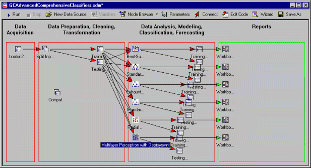
You can review the results for each model in the respective results nuggets in the Reports areas.
- During the initial research stage of your data mining project, you probably would want to review carefully the models, and how well they predict the response of interest.
- You can also double-click on each of the analysis nodes to select different types parameters for the respective analyses. In that case you can use the
Run
to
Node option (on the shortcut menu, or the
Run menu) to update only the selected node.
You can also now connect new data, marked for deployment, to the Compute Best Prediction from All Models node (the one that is not connected to anything at this point in the Data Preparation, Cleaning, Transformation area).
- Simply connect the Testing data (which was created as a random sample from the original input data source).
- Use option
Run
to node to compute the predicted classifications for each model.
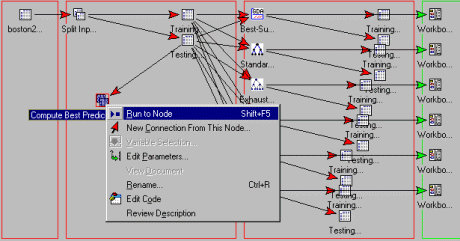
After a few seconds, the results spreadsheet with predictions is created as another node in the Data Preparation, Cleaning, Transformation area.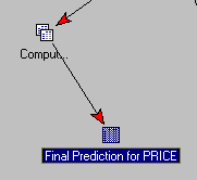
-
Review the final predictions by selecting
View Document
from the shortcut menu, after clicking on the
Final Prediction for PRICE
icon (which contains the predicted classifications for variable
PRICE from all models).
For example, you can compute a multiple histogram for the accuracy for each classifier (also reported in the
Final prediction for PRICE spreadsheet).
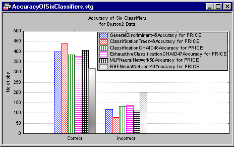
You could also look at the accuracy of classification, broken down by each category, and so on. In this case, it appears that all algorithms were reasonably accurate. By default, the Final Prediction spreadsheet will also contain a column with a voted classification from all classifiers. Predicted classification is often most accurate when it is based on multiple classification techniques, which are combined by voting (the predicted class that receives the most votes from participating models is the best prediction).
Shown below is the categorized histogram of the voted classifications by the observed classifications.
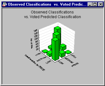
Clearly the voted classification produces excellent accuracy in the test sample. Remember that the test sample was randomly selected from the original data, and was not used to estimate the models (train the networks, etc.).
8. Prepare project for final customer deployment (in the "field").
Once deployment information is stored after training nodes marked with deployment, for classification or prediction (regression problems), you can save the entire project, and later retrieve that file to compute predicted values for new observations.
For example, a loan officer may want to predict credit risk based on the information provided on a loan application. The loan officer (end user, or customer) will not have to retrain the models in the current project again. Instead he or she can simply connect new data to the prediction node (usually labeled Compute Best Prediction From All Models) and proceed to process the new data. In fact, the data analyst who created the prediction model from training (learning) data can delete all computational (analysis) nodes from the project, and only leave a single node for computing predicted responses. In a sense, such projects are locked, (there is no risk of losing the deployment information due to accidentally starting a retraining of the models).
Advanced methods for deployment in the field
If you are familiar with Statistica Visual Basic (SVB), you can also consider writing a custom program that would further customize the user interface for the end-user of the deployed solution. If you review the function available for the Statistica DataMiner library in the SVB Object Browser, you can see that practically all aspects of the Statistica Data Miner user interface can be customized programmatically.
For example, you could attach the automatic application of a deployed solution to new data to a toolbar button so that a loan officer would only have to fill out a form with an applicant's data, click a button, and retrieve scores for credit risk and fraud probability.


