Example 2: Process Capability Analysis

Overview

This example is based on the same fictitious data set that was used in Example 1 - Pistons2.sta. To repeat, suppose you are producing piston rings for a small automotive engine; the target diameter of the piston rings is 74 millimeters (mm).

Unless the production process is under control, performing these analyses is rather pointless. Only when the process average and the process variability are stable can meaningful process capability indices be derived.

Assume for this example that the engineering specification limits for the process are ± .05 mm. Piston rings with a diameter smaller than 74 - .05 = 73.95 or greater than 74 + .05 = 74.05 mm are considered scrap and can potentially cause significant quality problems later on if used in automotive engines.

Specifying the analysis

Open the example data file Pistons2.sta, and start Process Capability Analysis:

1	Select the Home tab.
2	In the File group, click the Open arrow.
3	Select Open Examples to	The  Open a Statistica Data File dialog box displays.
4	Double-click the Datasets folder, and then open the data set.
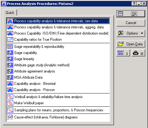
5	Next, on the Statistics tab, in the Industrial Statistics group, click Process Analysis to display the Process Analysis Procedures Startup Panel.	Process machine capability analysis & tolerance intervals, raw data is selected by default.
6	Click the OK button.	The Process Capability Analysis Setup--Raw Data dialog box displays.
7	On the Raw data tab, click the Variables button.	A standard variable selection dialog box displays
8	Select variable 1 (SAMPLE_1) as the Variable for the analyses.
9	Click the OK button.
10	On the Distribution tab, select the Normal and general non-normal (Pearson and Johnson fitting) option button.
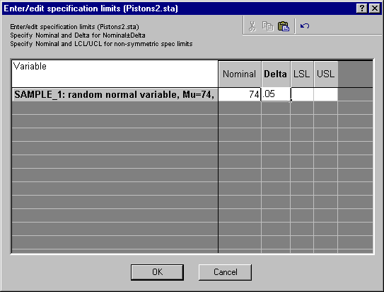
11	Click the OK button.	The Enter/edit specification limits dialog box displays
12	Enter 74 in the Nominal column and .05 in the Delta column.	The (nominal) target specification and the specification limits is specified.
13	Click the OK button.	The Process Capability Analysis--Normal and General Non-Normal Distribution dialog box displays

Reviewing the Results

The descriptive statistics for the piston diameters will be reviewed first.

1	Click on the Advanced, normal tab .
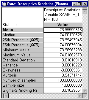
2	Click on the Descriptive statistics button.	The following spreadsheet displays.

The mean and standard deviation for the piston ring diameters are close to what is expected. Moreover, judging from the median, which is similar to the mean, and the skewness and kurtosis values, which are negligible in size, you would infer that the distribution of the piston ring diameters is probably close to normal.

You could also directly look at the frequency distribution via the Distribution & tests of normality button, which includes specific tests for normality.

Probability plots

Probability plots provide a quick visual check of how well the respective theoretical distribution (normal in this case) fits the observed data. These plots are described in the Introductory Overview.

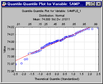
In quantile-quantile plots (or Q-Q plots for short), the observed values of a variable are plotted against the theoretical (for instance, normal) quantiles. If the points in that plot fall onto a straight line, then you conclude that the data follow the ( normal) distribution. You can produce that plot for the current data by clicking the Q-Q Normal distribution button.

With the exception of a few points in the tail areas, most points do fall onto a straight line, and you can be satisfied that the normal distribution assumption is probably met.

In probability-probability plots (or P-P plots for short) the observed cumulative distribution function is plotted against the theoretical cumulative distribution function. As in the Q-Q plot, if the data are follow the respective theoretical distribution (for instance, normal) then all data points will fall onto a straight line.

Here is the P-P plot for the current example data (click the P-P Normal distribution button).

Again, this plot is consistent with the assumption that the data are normally distributed.

Reviewing the summary histogram

Proceed now to the summary plot.

	Return to the Advanced, normal tab.
	Click the Summary histogram button.

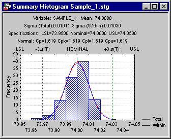
This plot is an example of a capable process (see Process (Machine) Capability Analysis Basic Overviews for a discussion of these plots, as well as a not-so-perfect example).

The summary histogram reports both sigma estimates and includes two normal distribution fits: one using the within-sample sigma and the other using total sigma. Within-sample sigma is used to calculate capability indices (e.g., Cpk) and, total sigma is used to compute other results (e.g., Ppk).

The specification limits are outside the effective process range (±3 sigma), and you can expect that very few piston rings were produced that fall outside the specification limits. Also, you can see that the normal distribution fits the observed data reasonably well. Now, look at the quantitative indices of process capability.

Process capability indices

The different process capability indices are explained in Process Capability Indices.

1	Click the Summary: Current variable button.
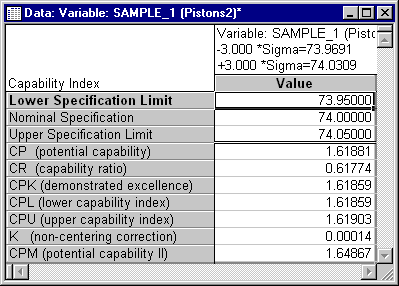
2	To display those indices for the current process, return to the Advanced, normal tab.	Two spreadsheets display, one containing the Capability Indices and another containing the Performance Indices. We will look at the Capability Indices. As expected, the Cp index (the ratio of the specification range over the process range) is greater than 1 (1.62), indicating a very capable process.
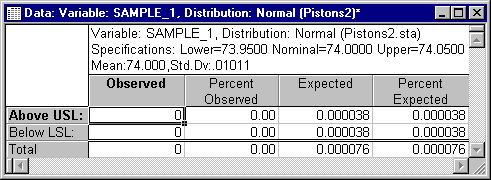
3	Now, return to the Advanced, normal tab and click the Number beyond specs (estimated & observed) button to see how many piston rings you can expect to produce that fall outside the specification limits.

There are no piston rings outside specification limits in this sample.

That is not surprising, considering that you would only expect to produce .000038 percent of such piston rings! Thus, you can conclude that the production process is, indeed, a capable process that yields high quality piston rings.

Tolerance limits

Obviously, most of the piston rings produced by the process are very close to specifications, but how close are they?

1

Because you have no reason to doubt that the piston ring diameters are normally distributed in the population of piston rings, click the Normal distribution tolerance limits button on the Tolerance limits tab to answer the above question.

You can select the sample size, confidence level, and percent population for the tolerance limits in the Compute limits based on group on the Tolerance limits tab.

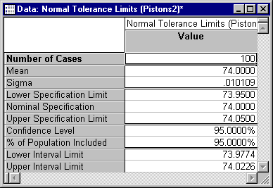
The results given in this spreadsheet are discussed in the Introductory Overviews. In summary, you can say with 95% confidence Confidence Level) that 95% of the population (% of Population Included) fall within the limits denoted in the spreadsheet as the Lower and Upper Interval Limit. You can play with the different parameters in this spreadsheet by using the options in the Compute limits based on group on the T

olerance limits

tab. For example, you can try different sample sizes or confidence limits, and see how the interval (tolerance) limits change as a result.

A Bad Example

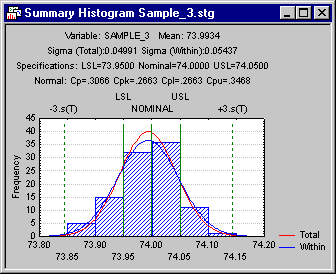
Before concluding this example, consider a bad process, that is, a process of low capability. For example, assume that due to machine wear, your sigma increases five-fold to .05. You may select variable 3 (Sample_3) in the data file Pistons2.sta which, as mentioned earlier, is actually a normal random variable with a mean of 74 and a sigma of .05.

1	To do this, click the Cancel button on the Process Capability Analysis - Normal and General Non-Normal Distribution dialog box.	The Startup Panel displays
2	Then, click the Variables button.	The standard variable selection dialog box displays.
3	Here, select variable 3 (Sample_3) as the Variable for the analyses and then click the OK button.
4	Now, click the OK button on the Startup Panel	The Enter/edit specification limits dialog box displays.
5	Specify the same sample specification limits as before - 74 in the Nominal column and .05 in the Delta column.
6	Click the OK button.	The Process Capability Analysis - Normal and General Non-Normal Distribution dialog box displays.
7	Click the Summary histogram button on the Advanced, normal tab.

Below is the resultant histogram.

Now the process range is much wider than the specification range. If you check the capability indices, you will find that C_p has dropped to .31 and, using the Number beyond specs (estimated & observed) button, you can expect approximately 32% of the piston rings to fall outside the specification limits. You would now conclude that there is trouble!

Remedies for bad processes

In practice, the use of carefully designed experiments, changing various parameters of the production process, usually leads quickly to significant improvement in the process capability.

The Experimental Design module offers a wide choice of such designs. In particular, Taguchi robust design techniques may be applicable and of great utility here.