Example 2: Variance Component Estimation for a Four-Way Mixed Factorial Design

This example illustrates restricted maximum likelihood (REML) estimation of variance components for a four-way mixed factorial design with multiple dependent variables. The example is based on a data set with four independent variables, a covariate, and three dependent variables. Two of the independent variables, Group and Gender, and their interaction are considered to have fixed effects. The remaining two independent variables, Time and Paid, and their interaction are considered to have random effects. All other interactions involving either Time or Paid are considered to be random effects. The Group and Gender factors have equal N's at each of their two levels. There are unequal N's for Time, with three levels, and Paid, with two levels. The data are contained in the file exp2.sta (a partial listing of this data file is shown below). Open this data file via the File - Open Examples menu; it is in the Datasets folder.

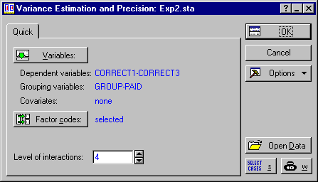
We will first perform the analysis without including the covariate in the model. To specify the design, select Variance Estimation and Precision from the Statistics menu to display the Variance Estimation and Precision Startup Panel. On the Quick tab, click the Variables button to display the standard variable selection dialog. Here, select variable Correct1, Correct2, and Correct3 as the Dependent variables, variables Time, Paid, Group, and Gender as Grouping variables, and then click the OK button. Because we want to fit all possible interaction terms, enter a 4 in the Levels of interactions field.

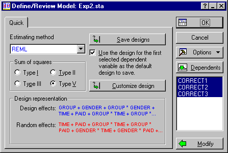
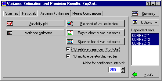
Click the OK button again to display the Define/Review Model dialog. Verify that all three dependent variables are selected in the Dependents list box and that REML and Type V are the selected Estimation method and Sums of squares type.

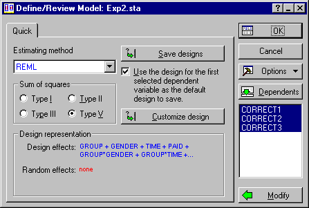
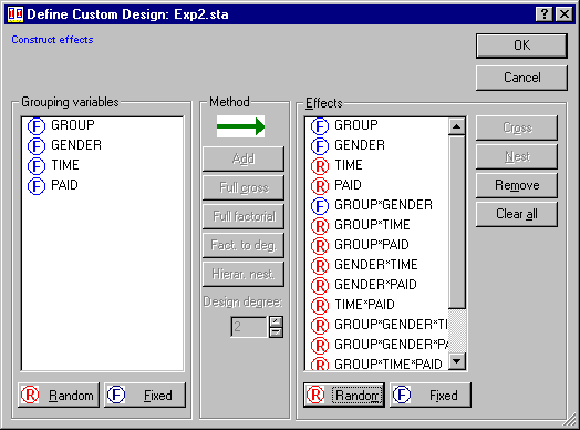
The default design representation is a full four-way factorial design; however, we need to specify fixed and random factors. Click the Customize design button to display the Define Custom Design dialog. In the Effects pane, select Time, Paid, and all interactions involving Time or Paid, then click the Random button. The Effects pane should look as shown below.

Click OK to return to the Define/Review Model dialog; notice that the list of Design effects and Random effects has been updated in the Design representation box.

Click OK again to display the Variance Estimation and Precision Results dialog.

To perform REML variance component estimation for the first dependent variable, first select Correct1 in the Dependent vars list box. Next, click on the Variance evaluation tab and click the Variance estimates button to display the Restricted Maximum Likelihood Estimates spreadsheet. The variance component estimates, standard errors, Wald statistics (Z value), degrees of freedom, cumulative values (Sum), percentages of total variation and relative standard deviation (RSD) are reported in this spreadsheet.

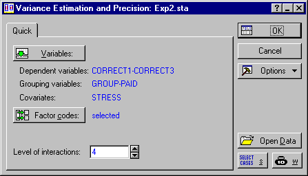
To perform the same analysis but with the covariate included in the model, return to the Variance Estimation and Precision Startup Panel by clicking the Modify buttons on the Variance Estimation and Precision Results dialog and the Define/Review Model dialog. On the Startup Panel, click the Variables button to again display the standard variable selection dialog (your previously chosen variables will still be selected) and then select Stress as the Covariate and click the OK button.

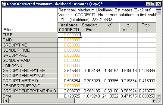
Next, click the OK button on the Startup Panel and on the Define/Review Model, click the Customize design button and specify the same effects as above (i.e., Group, Gender, and Group*Gender are fixed; all other effects are random). After specifying the design, click OK on the Define/Review Model dialog to display the Variance Estimation and Precision Results dialog. Once again, select Correct1 as the variable to be analyzed and on the Variance evaluation tab, click the Variance estimates button. The variance component estimates, standard errors, Wald statistics (Z value), degrees of freedom, cumulative values (Sum), percentages of total variation and relative standard deviation (RSD) for the model that includes the covariate, Stress, are reported in this spreadsheet.

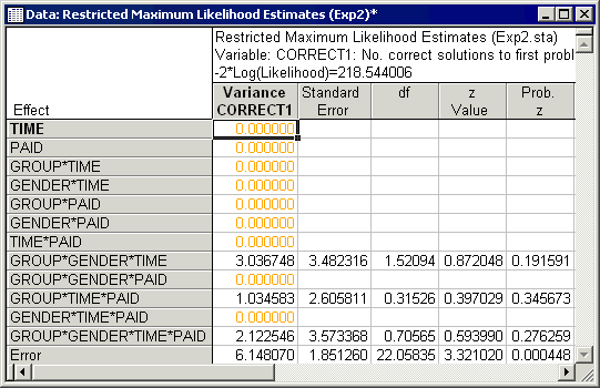
Comparing these results to those in the previous spreadsheet, where the covariate was not included in the model, has produced some notable differences. The negative of the natural logarithm of the likelihood decreased when the covariate was included in the model, indicating improvement of fit (the likelihood of the data can vary from zero to one, so minimizing the negative of the natural logarithm times the likelihood of the data amounts to maximizing the probability, or the likelihood, of the data). The estimate of the variance component for Error decreased when the covariate was included in the model, and the estimates of the other nonzero variance components increased. This shows the effects of reduction of the error on the estimation of variance components and the overall fit of the model.

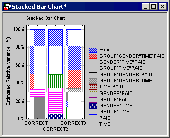
To graphically compare the relative variance components for all three dependent variables, select Correct1, Correct2, and Correct3 as the variables to be analyzed and select the Plot relative variances (% of total) check box.

Then click the Stacked bar of var. estimates button. This will produce a compound (or multiple) stacked bar plot which enable you to compare the magnitude of the nonzero variance components for each dependent variable.

This example has shown how to estimate variance components for complex mixed-model designs. Variance components were estimated for a four-way mixed factorial design. A covariate was also added to the model, to show the effects of reduction of error on the estimates of variance components. Graphical options were also described that aid in the comparison of variance component estimates across multiple dependent variables.

Implementation of maximum likelihood estimation algorithms is difficult (see, for example, Hemmerle & Hartley, 1973, and Jennrich & Sampson, 1976, for descriptions of these algorithms), and faulty implementation can lead to variance component estimates that lie outside the parameter space, converge prematurely to nonoptimal solutions, or give nonsensical results. Milliken and Johnson (1992) noted all of these problems with the commercial software packages they used to estimate variance components. In the Variance Estimation and Precision module (as in other Statistica modules), care has been taken to avoid these problems as much as possible. Note, for example, that for the analyses reported in this example, most Statistical packages do not give reasonable results.

 See also the Variance Estimation and Precision Index.