Special Topics Example 3 - Residuals Analysis

This example concerns the procedures in performing Residuals analysis. Residuals are the deviations of the observed values on the dependent variable from the predicted values, given the current model. The ANOVA models used in analyzing responses on the dependent variable in most of the programs in the Experimental Design module make certain assumptions about the distributions of residual (but not predicted) values on the dependent variable. These assumptions can be summarized by saying that the ANOVA model assumes normality, linearity, heteroscedasticity, and independence of residuals. These kinds of properties of the residuals for a dependent variable can be inspected using the options and selections available in the Experimental Design module.

Box and Draper (1987, page 205) report a study of the behavior of worsted yarn under cycles of repeated loading. (The same study is used as the basis for Example 3: Analyzing a 3**3 Full Factorial and Special Topics Example 4 - Box-Cox Transformation of a Dependent Variable.) The dependent variable of interest is the number of cycles to failure. Because of large variability in that variable, the log10 transformed dependent variable values were also considered. The data are contained in the data file Textile2.sta. The three factors included in the study are:

Factor	Low	Med	High
Length of specimen (mm)	250	300	350
Amplitude of load cycle (mm)	8	9	10
Load (g)	40	45	50

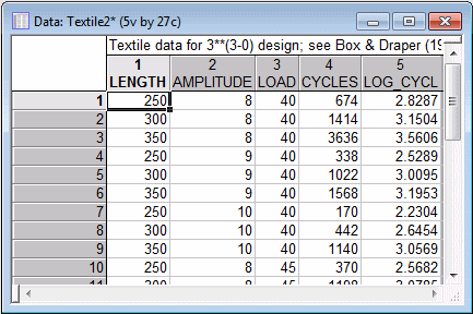
In this example, we will first look at the untransformed dependent variable values to illustrate a residual analysis indicating a faulty model and/or dependent variable. To begin the analysis, open the example data file Textile2.sta and start Experimental Design (DOE).

Ribbon bar. Select the Home tab. In the File group, click the Open arrow and from the menu, select Open Examples to display the Open a Statistica Data File dialog box. Double-click the Datasets folder, and open the Textile2.sta data set. Then, select the Statistics tab, and in the Industrial Statistics group, click DOE to display the Design & Analysis of Experiments Startup Panel.

Classic menus. On the File menu, select Open Examples  to display the Open a Statistica Data File dialog box. The Textile2.sta data file is located in the Datasets folder. Then, on the Statistics - Industrial Statistics & Six Sigma submenu, select Experimental Design (DOE) to display the Design & Analysis of Experiments Startup Panel.

In the Startup Panel, double-click 3**(k-p) and Box-Behnken designs to display the Design and Analysis of Experiments with Three-Level factors dialog box.

Select the Analyze design tab. Click the Variables button, and select Cycles and Log_Cycl as the Dependent variables; Length, Amplitud, and Load as the Indep (factors); and click OK.

Click OK in the Design and Analysis of Experiments with Three-Level factors dialog box to display the Analysis of an Experiment with Three-Level Factors dialog box.

Box and Draper (1987) began their residuals analysis by fitting the original (unlogged) dependent variable to the first degree polynomial equation. To reproduce the model coefficients reported by Box and Draper (1987, p. 214), select Cycles in the Variable drop-down list toward the top of the dialog box under the Summary box.

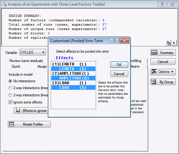
On the Model tab, select the No interactions option button, select the Ignore some effects check box, and in the Customized (Pooled) Error Term dialog box, highlight  the quadratic effects to pool them into the error term.

Click OK in the Customized (Pooled) Error Term dialog box.

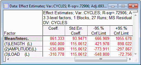
On either the Quick tab or the ANOVA/Effects tab, click the Summary: Effect estimates button to produce the Effect Estimates spreadsheet.

Shown above are the last four columns of the spreadsheet, with the coefficients for the recoded (-1,0,1) factor values. The column of t-values (not shown in the illustration above) shows that all three linear effects are highly significant.  

Select the Residual plots tab, and click the Histogram of residuals button. The histogram shows that the residuals are at least somewhat positively skewed.

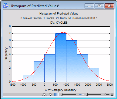
Now, click the Histogram of predicted values button. Here we see a hint of serious trouble; four of the predicted values are negative, which does not make physical sense on the number-of-cycles-to-failure dependent variable, although there is no clear evidence that the predicted values are negatively skewed.  

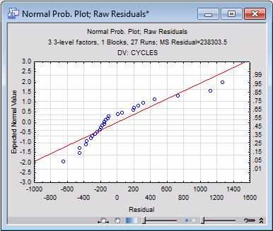
Next, click the Normal plot button in the Probability plots of residuals group box. You can see evidence of non-linearity in the plot of Expected Normal Values and corresponding probabilities against the Residuals, with very low and very high residuals falling below and moderate residuals falling above the straight line that is expected under the ANOVA model assumptions.  

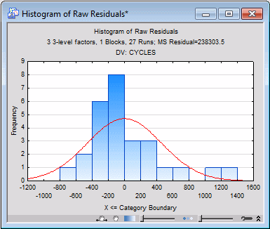
The Observed vs. predicted values plot shows the same pattern, and the Detrended normal plot shows the pattern even more clearly. The Predicted vs. residual values plot shows that the relation between the Residuals and Predicted Values clearly is not uniform, and the Observed vs residual values plot shows severe non-uniformity in the relation between the Observed values and Residuals. Fortunately, the uniformity of the Residuals vs. deleted residuals plot and the Residuals vs. case numbers plot provide no evidence of outliers or serial correlation in the observations, respectively, but nevertheless it is clear the residuals do not behave as would be expected if the usual ANOVA assumptions are met.

Perhaps most troubling of all, there is clear evidence that the cell variances on Cycles are strongly related to the cell means. It does take a little bit of ingenuity to make this determination, because there is only one case in each of the 27 cells of the 3 x 3 x 3 design, so the variance in each cell is, strictly speaking, undefined. However, the relations between marginal cell means and corresponding marginal cell standard deviations for pairs of factors collapsing across the third factor can be assessed.

For example, on the Means tab (or the Quick tab), in the under Observed marginal means group box, click the Display button to produce a spreadsheet with the marginal cell means and standard deviations for Length and Amplitude, collapsing across Load (highlight Length and Amplitude in the Compute marginal means for dialog box). If you were to perform a correlation between these marginal means and standard deviations it would be .96, or nearly perfect.

Select Log_Cycle in the Variable drop-down list, and repeat the analysis. You will find markedly lower correlations between marginal cell means and standard deviations, and the residuals plots reveal none of the irregularities identified above for the Cycles dependent variable. The log transformation produces markedly better behaved residuals.

One issue that remains, however, is whether it is better to transform a dependent variable with poorly-behaved residuals or to add higher-order terms to the prediction model to account for the non-linearity in the diagnostic plots of the residuals from the first degree polynomial (linear) model. For this example, Box and Draper (1987) present evidence that the former alternative is preferable.  

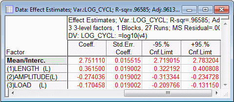
Shown below are the last four columns of the Effect estimates spreadsheet for the Log_Cycl  dependent variable (produced by clicking the Summary: Effect estimates button on either the Quick tab or the Anova/Effects tab), with the coefficients for the recoded (-1,0,1) factor values.

Of greatest interest is the R-square value of .96585, showing that virtually all of the variability in the transformed dependent variable is accounted for by the simple, first degree polynomial model. If you were to redo the analysis using the second degree polynomial model to fit the untransformed dependent variable Cycles (by selecting 2-way interactions (linear x linear) on the Model tab), the R-square value of .93788 is actually smaller. Thus, the greater complexity of a model with added higher order terms does not pay off in producing greater predictability of the untransformed dependent variable. Parsimony favors the adoption of the simpler model with the transformed dependent variable over the more complex model with the untransformed dependent variable, because in the latter case responses are explained no better than in the former.  

This example illustrates some of the procedures involved in conducting Residual analysis. Careful inspection of diagnostic plots and statistics can lead to more fruitful analyses and, at least sometimes, more interpretable results. For an additional example of diagnostic procedures for determining the need for transformation of the dependent variable, see Special Topics Example 4 - Box-Cox Transformation of a Dependent Variable.