Example 5: Seasonal Decomposition (Census Method I)
This example is based on a series reporting the monthly US total retail sales from 1953 to 1964. The data set is reported in Shiskin, Young, and Musgrave (1967) to illustrate the results of the X-11 (Census method II) seasonal adjustment procedure. In this example, the older Census method I seasonal decomposition method will be used to analyze this series; refer to the X-11 Seasonal Decomposition Example to see the results of the Census method II decomposition of this series.
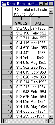
Select Time Series/Forecasting from the Statistics - Advanced Linear/Nonlinear Models menu to display the Time Series Analysis Startup Panel. Click the Variables button to display the standard variable selection dialog. Here, select variable Sales and then click the OK button. Then, click the Seasonal decomposition (Census 1) button to display the Ratios-To-Moving Averages Classical Seasonal Decomposition (Census Method I) dialog.
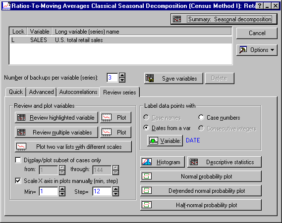
Now, click the Plot button next to the Review highlighted variable button.
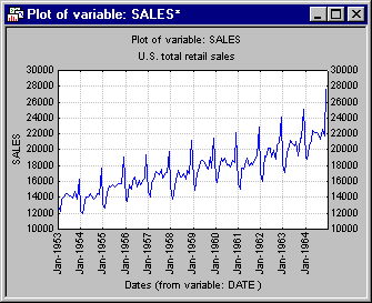
The retail sales show an upward trend and clear seasonal fluctuation. As described in the Introductory Overview, the goal of seasonal decomposition in general is to derive estimates of the seasonal, trend-/cycle, and irregular components that make up the series. The seasonal component can be used to compute a seasonally adjusted series, that is, an estimate of the series after removing seasonal fluctuations.
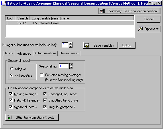
You are now ready to perform the analysis. Click the Summary: Seasonal decomposition button, and the result spreadsheet with all series will be displayed.

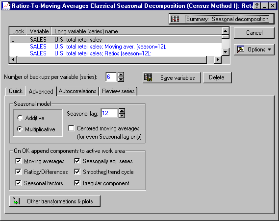
Plot the components that were extracted. Highlight (click on) the Seasonal factors series in the active work area and then click the Plot button next to the Review highlighted variable button on the Review series tab.
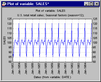
This is the stable seasonal variability that was extracted from the series. This seasonal component can be used to adjust the original series (i.e., it is either subtracted from the original series if the model is additive, or it is divided into the original series if the model is multiplicative).
Click the Plot button next to the Review multiple variables button to display the Select variables for the Spreadsheet/plot dialog. Select the original series Sales and the Adjusted series (use the CTRL key to make discontinuous selections) and then click the OK button to produce the plot.
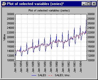
As you can see, the adjusted series shows no seasonal fluctuation any more. One can further smooth that series in order to remove the remaining random (irregular) fluctuations.
The smoothed seasonally adjusted series represents the Trend/Cycle component, because it will show the overall trend and cycles in the series (the cycle component is different from the seasonal component in that cycles usually last longer than a single seasonal period, and they occur at irregular intervals). Shown below is the plot of the trend/cycle and seasonally adjusted series. (Click the Plot button next to the Review multiple variables button and select the trend/cycle and seasonally adjusted series.)
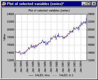
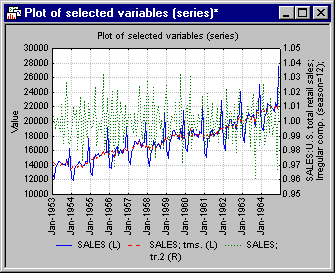
Finally, look at the irregular series with the residual fluctuations in the series. The residuals along with the original and seasonally adjusted series can be shown.
Click the Plot two var lists with different scales button and select the original and seasonally adjusted series for the Variables (series) to be plotted against left-Y axis, and select the Irregular series for the Variables (series) to be plotted against right-Y axis in the resulting Select variables for plot/spreadsheet dialog.
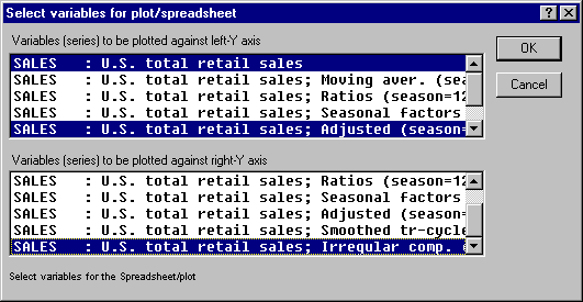
Click the OK button to produce the summary plot.
See also, Time Series Analysis Index.