Example 3: Ordinal Multinomial Linear Model with Probit Link
This example is based on the example data file Ideol.sta (see Agresti, 1996, p. 214). The data are from a 1991 general social survey, and describe the relationship between respondents' political ideology and political party affiliation. Political ideology was measured on a five-point scale, from 1-Very liberal to 5-Very conservative. Specifically, the data file contains the following variables:
Party: Respondents' party affiliation, Democratic or Republican
Ideology: Respondents' ideology (ordinal categorical dependent (response) variable with 5 categories)
Count: Number of respondents in the respective cell in the table (that is combination of Party and Ideology)
Since political Ideology was measured on an ordinal (5-point) scale, an ordinal multinomial model with a probit link is fitted. In the ordinal multinomial model, common slopes of predictors but different intercept terms are assumed. See McCullagh and Nelder (1989), Hosmer and Lemeshow (1989), and Agresti (1996) for detailed discussions of the ordinal multinomial linear model.
Open the Ideol.sta data file:
Ribbon bar. Select the Home tab. In the File group, click the Open arrow and from the menu, select Open Examples. The Open a Statistica Data File dialog is displayed. Ideol.sta is located in the Datasets folder.
Classic menus. From the File menu, select Open Examples to display the Open a Statistica Data File dialog; Ideol.sta is located in the Datasets folder.
Ribbon bar. Select the Statistics tab. In the Advanced/Multivariate group, click Advanced Models and from the drop-down list, select Generalized Linear/Nonlinear to display the Generalized Linear/Nonlinear Models Startup Panel.
Classic menus. From the Statistics - Advanced Linear/Nonlinear Models submenu, select Generalized Linear/Nonlinear Models to display the Generalized Linear/Nonlinear Models Startup Panel.
Select the Advanced tab. Select One-way ANOVA as the Type of analysis, Quick specs dialog as the Specification method, Ordinal multinomial as the Distribution, and Probit as the Link functions. Then click the OK button to display the GLZ One-Way ANOVA Quick Specs dialog.
On the Quick tab, click the Variables button to display the standard variable selection dialog. Select Ideology as the Dependent (response) variable, Party as the Categorical predictor, and Count as the Count Variable, and then click the OK button.
You can use all other default specifications, so click the OK button in the GLZ One-Way ANOVA Quick Specs dialog to display the GLZ -- Results dialog.
If you want to run this example using GLZ Syntax, you can run the following syntax program from the GLZ Analysis Syntax Editor dialog (see Methods for Specifying Designs).

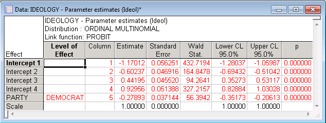
By examining the confidence intervals for the parameter estimates, and how they overlap, you can determine which parameters are significantly different from each other.

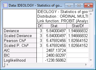
In this example, the values of the ratios of the statistics over the degrees of freedom are larger than one. This may be evidence of overdispersion (see McCullagh and Nelder, 1989, p. 124-128, p. 174). To address this problem, you can select the Overdispersion check box and choose either the Pearson Chi2 or Deviance option button for the estimate of the dispersion parameter (that is, to specify a scale parameter other than 1.0). Changing the overdispersion parameter affects the computation (values) of the parameter variances and covariance and the model likelihood, and all related statistics (example, standard errors, prediction errors). For details, refer to McCullagh and Nelder (1989).