Example 4: Comparing Two Learning Curves
This example demonstrates how one can evaluate differences in the regression model across groups. The data set for this example is again based on Neter, Wasserman, and Kutner (1985, page 484) and is contained in the file Learning.sta. Open this data file by selecting Open Examples from the File menu (classic toolbar) or by selecting Open Examples from the Open menu on the Home tab (ribbon bar); it is in the Datasets folder.
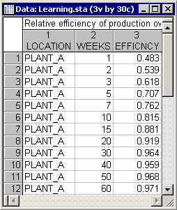
Suppose you are about to introduce a new electronics product that will be manufactured in two different plants: Plant_A and Plant_B. You may know that plant B is a more modern facility; therefore, you would expect that plant to adapt to the new production process more quickly. To study the efficiency of the two plants, the ratio of the per-unit-production cost that would be expected in a modern facility after learning has occurred over the actual per-unit-production cost for selected weeks over a 90-week span was recorded in the variable Efficncy.
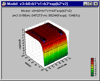
Neter et al. fit the following model to these data:
y = b0 + b1*xg + b3*exp(b2*x)
In this model, xg denotes a coding variable that identifies each plant (plant A = 0; plant B = 1; the same codes are used in Learning.sta). If parameter b1 is significant then it can be concluded that there is a significant constant (or additive) difference between groups.
Select Nonlinear Estimation from the Statistics - Advanced Linear/Nonlinear Models menu to display the Nonlinear Estimation Startup Panel. Double-click the User-specified regression, custom loss function option in the Startup Panel. Click the Function to be estimated & loss function button in the User-Specified Regression, Custom Loss dialog to display the Estimated function and loss function dialog. Now enter the regression equation: v3=b0+b1*v1+b3*exp(b2*v2) in the Estimated function box and accept the default ordinary least squares loss function in the Loss function box.
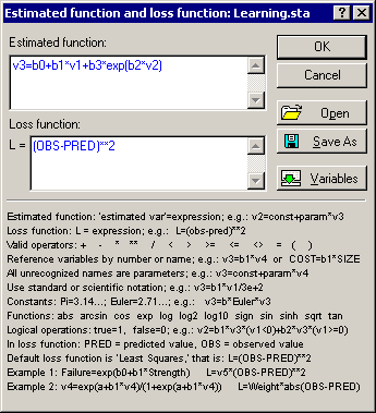
In this case, the variables have been referenced via the Vxxx convention (where xxx is a variable number), and bx was used to refer to the parameters. Thus, typing in this formula is not that difficult (i.e., lengthy). However, note that you can also easily save the formulas via the Save As button and open them at a later time using the Open button.
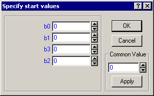
Now select the Rosenbrock and quasi-Newton method from the Estimation method drop-down box and also select the Asymptotic standard errors check box on the Advanced tab. Then, click the Start values button to display the Specify start values dialog. Set all initial parameter estimates to 0 by entering 0 in the Common Value box and clicking the Apply button.
Click the OK button in this dialog and again in the Model Estimation dialog to begin the estimation. Note that on slower computers, this estimation may take a while. In this case, instead of choosing the method described here, enter start values that are similar but not identical to the final parameters and then use Quasi-Newton for estimating the parameters; this will speed up the estimation.
After about 8 iterations, the Rosenbrock method will quit and Statistica will continue with the Quasi-Newton method, starting where the Rosenbrock method left off. After only 11 additional Quasi-Newton iterations, the estimation process will converge and the Results dialog will appear.
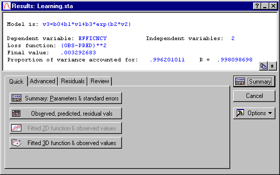
Now, look at the parameter estimates by clicking the Summary: Parameters & standard error button.
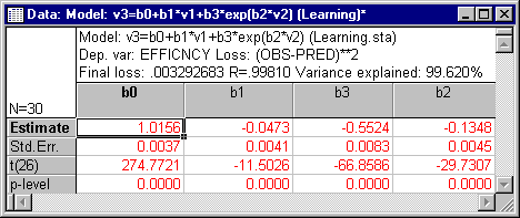
The crucial parameter b1 is highly significant (p<.001); thus, you can conclude that the two plants do indeed differ in their efficiency. Return to the Results dialog and click the Normal probability plot of residuals button on the Residuals tab to make sure that the model is appropriate.
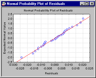
All points are very close to the line denoting the normal distribution; therefore, it can be concluded that the model is quite appropriate.