Example 4: Weibull and Reliability/Failure Time Analysis
This example is based on a data set presented in Dodson (1994, Table 2.5). No specific information is provided regarding the origin of these data, however, the data set is an example of multiple-censored failure time data. The example data are available in the example data file Dodson25.sta. Open this data file via the File - Open Examples menu; it is in the Datasets folder.
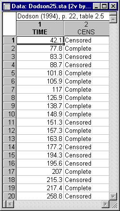
The goal of the analysis is to fit the Weibull distribution to these data, and to estimate the percentiles of the reliability function.
On the Raw data tab, click the Variables (failure times & censoring indicator) button to display a standard variable selection dialog. Select variable Time as the variable with Failure times, variable Cens as the Censoring indicator variable, and then click the OK button.
Now, double-click the Code for complete responses (failures) field to display the Variable 2 dialog. Select Complete and then click the OK button. In the same manner, select Censored as the Code for censored responses.
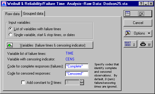
Then click the OK button to start the analysis.
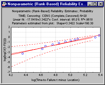
This plot shows the observed failure data, the linear fit line (in blue), the 95% nonparametric confidence interval for the reliability (i.e., the log-log transformation, as indicated by the y-axis label in the plot shown above; the confidence interval is indicated by the red dotted lines), and the center (50th percentile) of the nonparametric confidence interval (indicated by the dashed red line). As briefly described in the Introductory Overview, you can estimate the shape and scale parameters from the slope and intercept of the linear fit line in this plot; specifically, the shape parameter is equal to the slope of the linear fit-line, and the scale parameter can be estimated as exp(-intercept/slope). The resultant estimates for this specific plot, 3.34 and 190.3 for the Shape and Scale parameters, respectively, are very similar to the maximum likelihood parameter estimates. Also, because the points in this plot are well represented by the fitted line (R2 is equal to .96), we have reason to believe that the Weibull distribution with these parameters provides an adequate fit to the data.

Refer to the Introductory Overview for additional details about these tests.
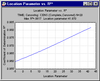
It is apparent from this plot that the R2 value steadily increases up to a value very close to the smallest (censored) failure time recorded in the data. (In other cases, you may see a curve with a single peak; see, for example, Figure 2.6 in Dodson, 1994.) Next, on the Advanced tab, select the ML location, shape, scale parameters option button to compute the maximum likelihood estimates for the three-parameter Weibull distribution; then click the Summary: Parameters button to review the parameters and their standard errors.
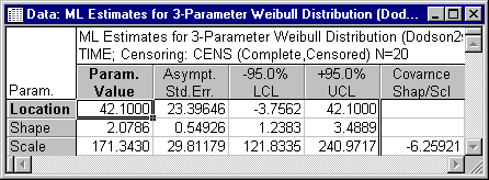
Evidently, even though the Location parameter is estimated as 42.1, the 95% confidence limits include 0, and therefore, we will accept the (simpler) two-parameter model, with the location parameter equal to zero. Select the ML shape & scale parameters option button and then enter 0 in the Offset (threshold/location) box. Next, click the Recompute button and then click the Summary: Parameters button again to compute the maximum likelihood parameter estimates for the two-parameter distribution.
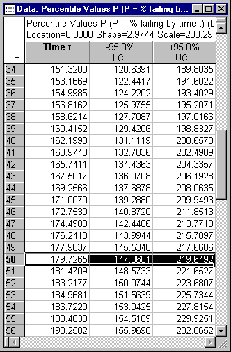
The spreadsheet shows the percentile values in one percent increments, i.e., for percentile 1, 2, 3, 4, and so on. For example, for the 50th percentile, the time value is equal to 179.73, with a 95% confidence interval from 147.06 to 219.65. In other words, 50% of all items can be expected to have failed prior to t=179.73 (with the respective confidence interval).