FORECAST_SEASONAL: Using Triple Exponential Smoothing
Triple exponential smoothing produces an exponential moving average that takes into account the tendency of data to repeat itself in intervals over time. For example, sales data that is growing and in which 25% of sales always occur during December contains both trend and seasonality. Triple exponential smoothing takes both the trend and seasonality into account by using three equations with three constants.
For triple exponential smoothing you, need to know the number of data points in each time period (designated as L in the following equations). To account for the seasonality, a seasonal index is calculated. The data is divided by the prior season index and then used in calculating the smoothed average.
- The first equation
accounts for the current time period, and is a weighted average
of the current data value divided by the seasonal factor and the
prior average adjusted for the trend for the previous period. The
weight constant is k:
SEASONAL(t) = k * (datavalue(t)/I(t-L)) + (1-k) * (SEASONAL(t-1) + b(t-1))
- The second equation
is the calculated trend value, and is a weighted average of the
difference between the current and previous average and the trend
for the previous time period. b(t) represents the average
trend. The weight constant is g:
b(t) = g * (SEASONAL(t)-SEASONAL(t-1)) + (1-g) * (b(t-1))
- The third equation
is the calculated seasonal index, and is a weighted average of the
current data value divided by the current average and the seasonal
index for the previous season. I(t) represents the average
seasonal coefficient. The weight constant is p:
I(t) = p * (datavalue(t)/SEASONAL(t)) + (1 - p) * I(t-L)
These equations are solved to derive the triple smoothed average. The first smoothed average is set to the first data value. Initial values for the seasonality factors are calculated based on the maximum number of full periods of data in the data source, while the initial trend is calculated based on two periods of data. These values are calculated with the following steps:
- The initial trend
factor is calculated by the following formula:
b(0) = (1/L) ((y(L+1)-y(1))/L + (y(L+2)-y(2))/L + ... + (y(2L) -
y(L))/L )
- The calculation of
the initial seasonality factor is based on the average of the data values
within each period, A(j) (1<=j<=N):
A(j) = ( y((j-1)L+1) + y((j-1)L+2) + ... + y(jL) ) / L
- Then, the initial
periodicity factor is given by the following formula, where N is
the number of full periods available in the data, L is the number
of points per period and n is a point within the period (1<=
n <= L):
I(n) = ( y(n)/A(1) + y(L+n)/A(2) + ... + y((N-1)L+n)/A(N) ) / N
The three constants must be chosen carefully. The best results are usually obtained by choosing the constants to minimize the mean-squared error (MSE) between the data values and the calculated averages. Varying the values of npoint1 and npoint2 affect the results, and some values may produce a better approximation. To search for a better approximation, you may want to find values that minimize the MSE.
The equation used to forecast beyond the last data point with triple exponential smoothing is:
forecast(t+m) = (SEASONAL(t) + m * b(t)) / I(t-L+MOD(m/L))
where:
Is the number of periods ahead for the forecast.
Calculate a Triple Exponential Smoothing Column
FORECAST_SEASONAL(display, infield,
interval, npredict, nperiod, npoint1, npoint2, npoint3)
where:
Keyword
Specifies which values to display for rows of output that represent existing data. Valid values are:
- INPUT_FIELD. This displays the original field values for rows that represent existing data.
- MODEL_DATA. This displays the calculated values for rows that represent existing data.
Is any numeric field. It can be the same field as the result field, or a different field. It cannot be a date-time field or a numeric field with date display options.
Is the increment to add to each sort field value (after the last data point) to create the next value. This must be a positive integer. To sort in descending order, use the BY HIGHEST phrase. The result of adding this number to the sort field values is converted to the same format as the sort field.
For date fields, the minimal component in the format determines how the number is interpreted. For example, if the format is YMD, MDY, or DMY, an interval value of 2 is interpreted as meaning two days. If the format is YM, the 2 is interpreted as meaning two months.
Is the number of predictions for FORECAST to calculate. It must be an integer greater than or equal to zero. Zero indicates that you do not want predictions, and is only supported with a non-recursive FORECAST. For the SEASONAL method, npredict is the number of periods to calculate. The number of points generated is:
nperiod * npredict
For the SEASONAL method, is a positive whole number that specifies the number of data points in a period.
For SEASONAL, this number is used to calculate the weights for each component in the average. This value must be a positive whole number. The weight, k, is calculated by the following formula:
k=2/(1+npoint1)
For SEASONAL, this positive whole number is used to calculate the weights for each term in the trend. The weight, g, is calculated by the following formula:
g=2/(1+npoint2)
For SEASONAL, this positive whole number is used to calculate the weights for each term in the seasonal adjustment. The weight, p, is calculated by the following formula:
p=2/(1+npoint3)
Calculating a Triple Exponential Smoothing Column
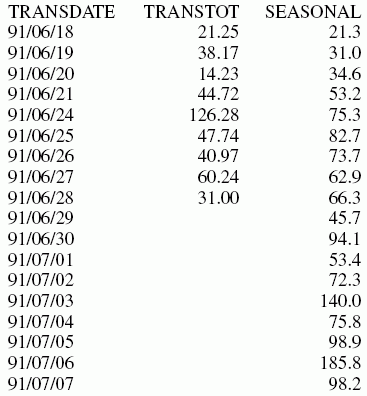
In the following, the data has seasonality but no trend. Therefore, npoint2 is set high (1000) to make the trend factor negligible in the calculation:
TABLE FILE VIDEOTRK
SUM TRANSTOT
COMPUTE SEASONAL/D10.1 = FORECAST_SEASONAL(MODEL_DATA,TRANSTOT,1,3,3,3,1000,1);
BY TRANSDATE
WHERE TRANSDATE NE '19910617'
ON TABLE SET STYLE *
GRID=OFF,$
ENDSTYLE
END
In the output, npredict is 3. Therefore, three periods (nine points, nperiod * npredict) are generated.
