Procedure: How to Run Regression Models
After you create a Data Flow, you can select from various regression model algorithms to run against your data set.
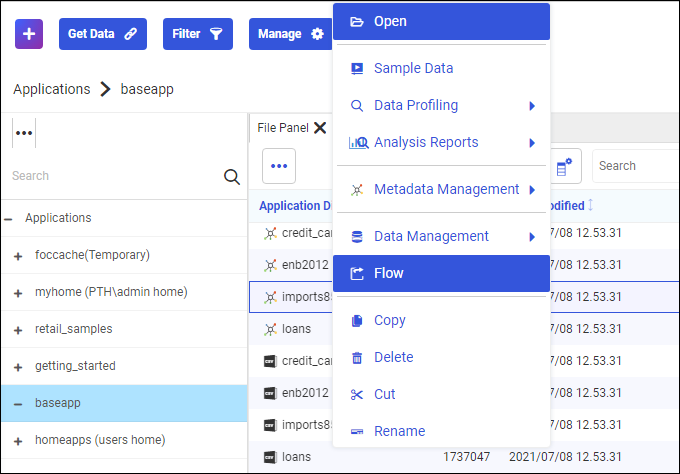
- From the Applications page, right-click a data set, click New, and select Flow, as shown in the following image.
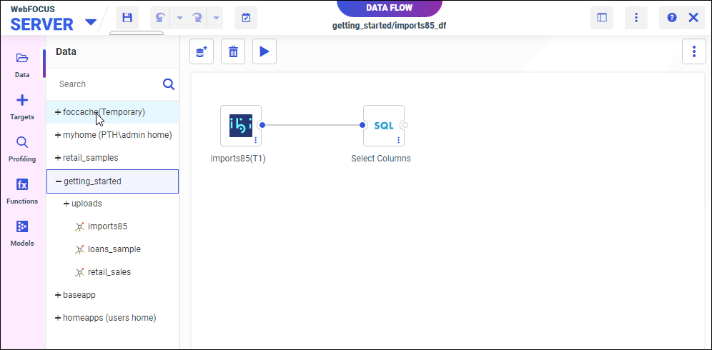
The Data Flow opens, as shown in the following image.
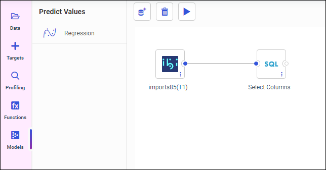
- From the side panel, click Models.
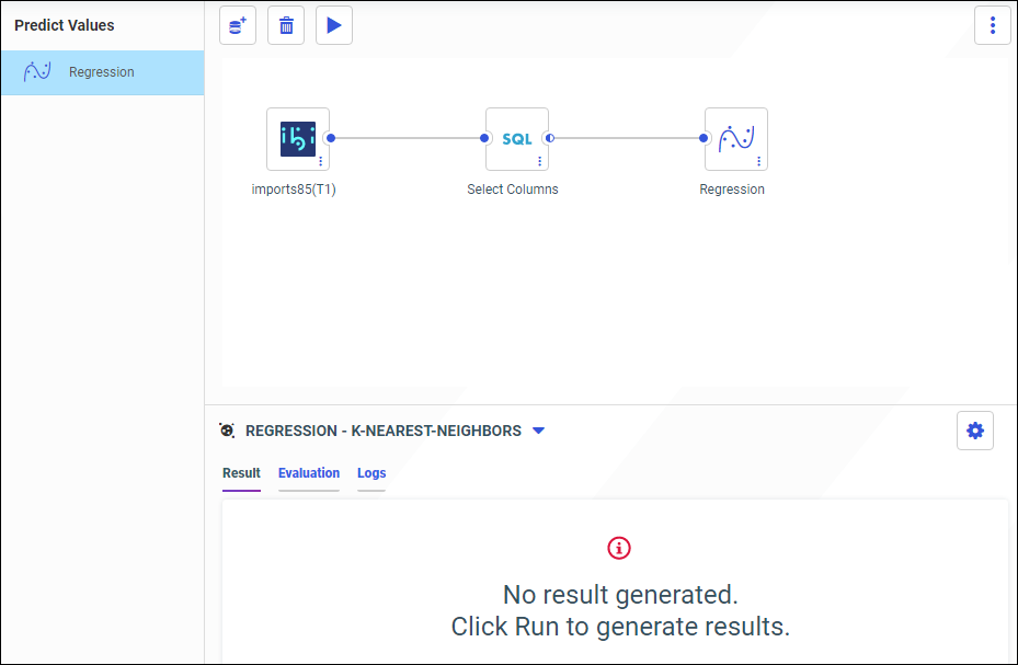
The Predict Values panel opens, as shown in the following image.
The following regression model algorithms display within the Regression module:
- Random Forest
- K-Nearest-Neighbors
- Polynomial
- Extreme Gradient Boosting
- Double-click or drag and drop the regression model to the canvas. The Configure Regression dialog box displays, as shown in
the following image.
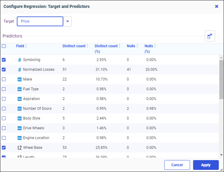
You can click the Target dropdown menu to select a different target. All numeric Field measures are selected by default as Predictors. You can add or remove Predictors by selecting or unselecting the check boxes.
- Click Apply.
Your selected model type appears on the dataflow canvas, as shown in the following image.
To edit your model target and predictors, right-click the canvas Regression node, select Edit Settings, and then select Target and Predictors.
To edit your model hyperparameters, right-click the canvas Regression node, select Edit Settings, select Hyperparameters, and then select a model algorithm. Hyperparameters have default values that are unique to each model.
- Click the Run icon
 to train your model.
The Compare Model Evaluation Results dialog opens, as shown in the following image.
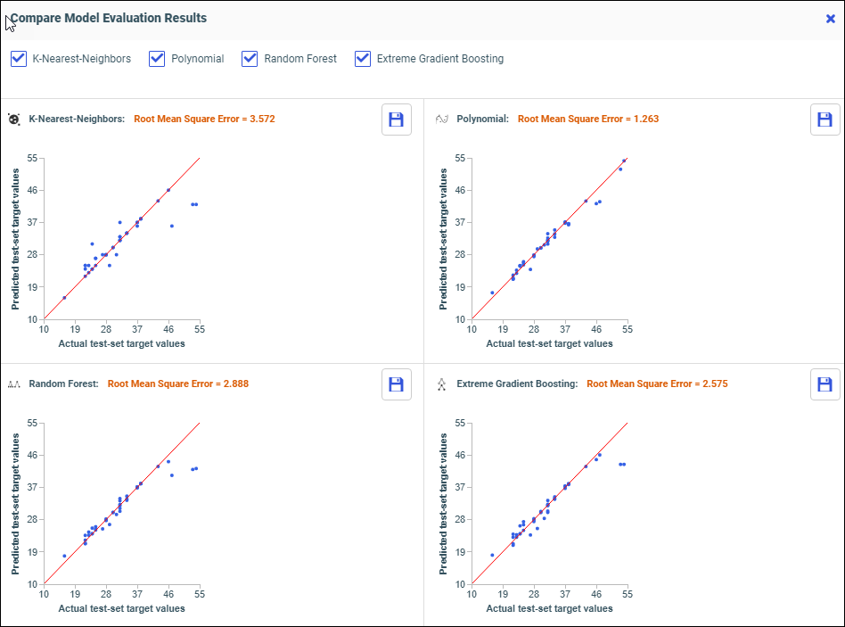
The regression model algorithms run in parallel. This allows you to easily compare results and determine which model is best to save.
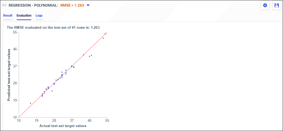
The best model has the lowest Root Mean Square Error value, and a scatter plot with dots closest to the red line. In this example, the Polynomial model has the best results.
You can filter which model comparisons you want to see by selecting or deselecting the model check boxes.
You can save a model by clicking its Save icon.
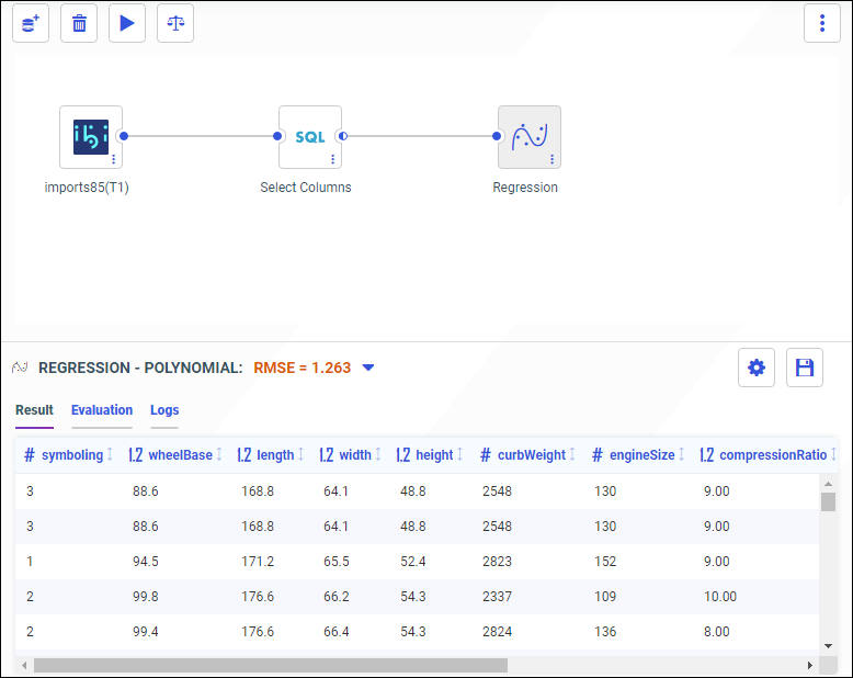
Close the Compare Model Evaluation Results dialog box to return to the canvas, as shown in the following image.
To open the Compare dialog box, click the Compare icon
 on the canvas toolbar.
You can select different model algorithms from the Regression drop-down menu. The best model displays by default. Models display in the following tabs.
- Result. A preview of the first 50 rows of your new data set.
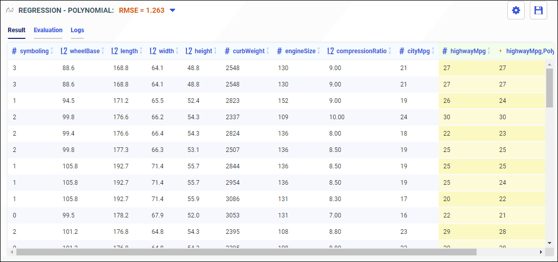
Target and predicted columns are highlighted yellow, as shown in the following image.
- Evaluation. A report that demonstrates the accuracy of the selected model.
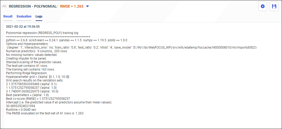
- Logs. A report that includes the performance metrics and hyperparameter values.
- Feature Importances. The most important features in your data set.

Note: Feature Importances is available for the Random Forest model only.
- Result. A preview of the first 50 rows of your new data set.
- Click the Save icon to save your model.
The Save dialog opens, as shown in the following image.
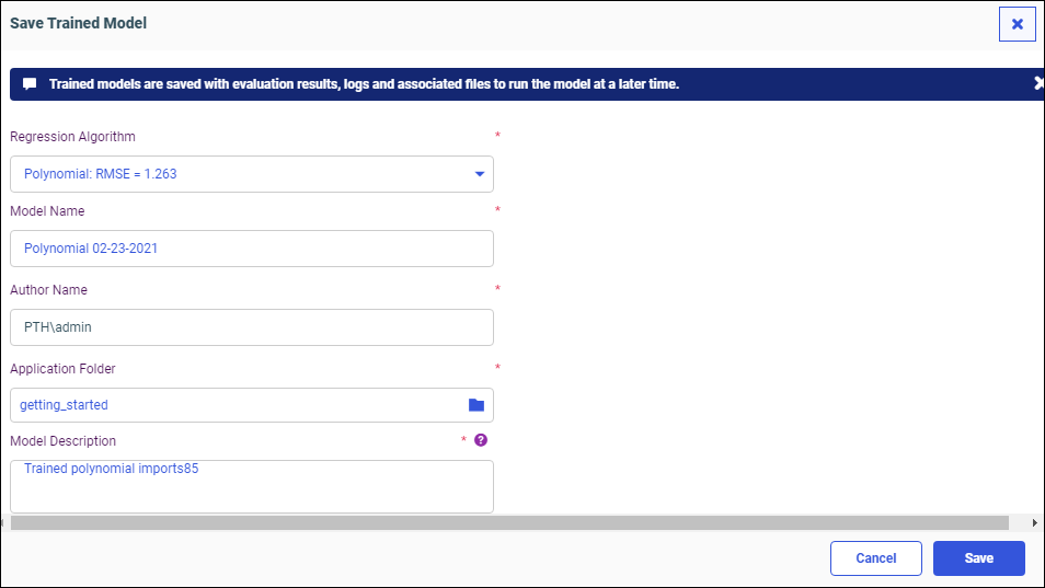
You can change the model algorithm, name, or location, and add a description.
- Click Save.
Your model is saved to your selected folder location, as shown in the following image.
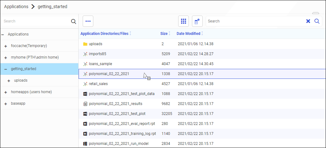
Trained models are saved with evaluation results, logs, and associated files, to run the model at a later time.