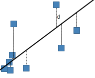
Curve fit models

There are several different models available for curve fitting. The various models are briefly explained here.

Straight line

The straight line fit is calculated by choosing the line that minimizes the least square sum of the vertical distance d, of all the selected markers (see picture below) by using the following equation:

where a is the intercept and b is the slope.

For example, you could plot days along the X-axis and have one marker for each day. The distance between the markers along the X-axis is the same, thus making straight line fit appropriate.

Logarithmic

The logarithmic fit calculates the least squares fit through points by using the following equation:

where a and b are constants and ln is the natural logarithm function. This model requires that x>0 for all data points. Spotfire uses a nonlinear regression method for this calculation. This will result in better accuracy of the calculation compared to using linear regression on transformed values only.

Exponential

The exponential fit calculates the least squares fit through points by using the following equation:

where a and b are constants, and e is the base of the natural logarithm.

Exponential models are commonly used in biological applications, for example, for exponential growth of bacteria. Spotfire uses a nonlinear regression method for this calculation. This will result in better accuracy of the calculation compared to using linear regression on transformed values only.

Power

The Power fit calculates the least squares fit through points by using the following equation:

where a and b are constants. This model requires that x>0 for all data points, and either that all y>0 or all y<0. Spotfire uses a nonlinear regression method for this calculation. This will result in better accuracy of the calculation compared to using linear regression on transformed values only.

Logistic regression

The logistic regression fit is a dose response ("IC50") model, also known as sigmoidal dose response. The four parameter logistic model is the most important one.

Dose-response curves describe the relationship between response to drug treatment and drug dose or concentration. These types of curves are often semi-logarithmic, with log (drug concentration) on the X-axis. On the Y-axis, you can show measurements of enzyme activity, accumulation of an intracellular second messenger or measurements of heart rate or muscle contraction.

Note: The logistic regression model of Spotfire is implemented with a setting where you can select whether or not to assume that X is log10-transformed. The default setting is a selected check box, which means that if your input data is not logarithmic, you should make sure to clear Assume that X is log10-transformed when defining the curve. You might also want to select the Log scale check box in the X-axis section of the visualization properties, to show the values on a logarithmic scale.

Log10-transformed X-values

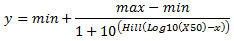
The logistic regression on logged X-values fit uses the following equation:

The LoggedX50 value is interpreted as the Log10(X50). For example, if the H30+ concentration at IC50 has a pH of 3, then the LoggedX50 = -3.

Note: With this model, it is the logged X50 values that are estimated and not the actual X50.

Non-logarithmic X-values

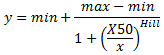
The logistic regression fit when not assuming logged X-values uses the following equation:

where min and max are the lower and upper asymptotes of the curve, Hill is the slope of the curve at its midpoint and X50 is the x-coordinate of the inflection point (x, y). This model requires that x>0 for all data points and that you use at least four records to calculate the curve.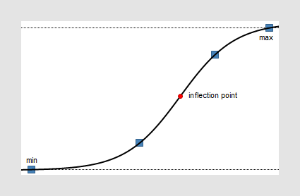

Polynomial

The polynomial curve fit calculates the least squares fit through points by using the following equation:

where a0, a1, a2, etc., are constants. The default order is a 2nd order polynomial, but you can change the degree in the settings for the curve. This model requires that you use at least three markers to calculate the curve for a 2nd order polynomial model, and four markers for a 3rd order polynomial, and so on.

If you have a low number of unique x-values, a polynomial curve can be calculated in an unlimited number of ways. This means that you might end up with a curve that does not look as expected. If this happens, you probably should not apply this model to your data.

Some of the models have been partially solved by using the LAPACK software package, see References.

Gaussian

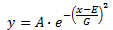
The Gaussian curve fit calculates a bell curve suitable to describe normal distributions using the following equation:

where A is the amplitude (height) of the curve, E is the position of the center of the curve and G is the width.

In Spotfire, you have the possibility to let the application calculate values on the parameters A, E and G automatically from the available data by leaving the curve parameter fields blank. You can also specify one or more of the parameters yourself.

Holt-Winters forecast

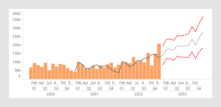
The Holt-Winters Forecast uses Spotfire® Enterprise Runtime for R (a/k/a TERR™) to compute the Holt-Winters filtering of a time series or anything that can be coerced to a time series. This is an exponentially weighted moving average filter of the level, trend, and seasonal components of a time series. The smoothing parameters are chosen to minimize the sum of the squared one-step ahead prediction errors.

The output of a Holt-Winters Forecast is three different curves: a fitted curve showing the general variation of the measure of interest, a forecast curve predicting the future trend and a confidence interval showing how the insecurity increases the further away from the known values the prediction reaches.

You can switch on or hide the three curves separately from Visualization properties.

Tip: In the installed client, you can right-click on a suitable visualization and select Forecast to add a Holt-Winters forecast directly.

Note: TERR and open-source R return different prediction intervals for multiplicative seasonal models. TERR assumes that the seasonal and error components are multiplicative in effect and it uses the formula for prediction variance found in section 6.4.2 of Hyndman, et al, 2008. See the references listed in the References section.

When defining a Holt-Winters Forecast, you can specify the following:

Level (alpha) – Specifies how to smooth the level component of the time series.
The level (alpha) parameter must be larger than 0 but not larger than 1.

A small value means that older values in the X direction are weighted more heavily.

Values near 1.0 mean that the latest value has more weight.
Trend (beta) – Specifies how to smooth the trend component of the time series.
The trend (beta) parameter must be in the interval of 0-1.

A small value means that older values in X direction are weighted more heavily.

Values near 1.0 mean that the latest value has more weight.
Seasonal (gamma) – Specifies how to smooth the seasonal component of the time series.
The seasonal (gamma) parameter must be in the interval of 0-1.

A small value means that older values in X direction are weighted more heavily.

Values near 1.0 mean that the latest value has more weight.

Use the drop-down list to specify how the seasonal component should interact with the other components:

Additive (default) indicates that X is modeled as level + trend + seasonal.

Multiplicative indicates the model is (level + trend) * seasonal.
Frequency – Only applicable when a Seasonal (gamma) component is included in the model.
Specifies the number of seasonal periods to use to compute start values, that is, the number of observations per sampling period. For example, monthly data have a frequency of 12. The frequency must be greater than 1 to fit a seasonal component.
Time points ahead – Specifies the number of time points (nodes) into the future at which to predict the values of the time series.
If the visualization shows months, then the time points ahead equals the number of months forward to predict. If the visualization shows years, then the time points ahead represents the number of years forward to predict.
Confidence level – Specifies the confidence level. This should be a number larger than 0 but not larger than 1.
Allow replacement of empty values – Allows you to replace empty values by interpolating the adjacent values. Note that two missing data points in a row cannot be interpolated.

You can specify a frequency or the time points ahead, either using a fixed number or by using a property value, selected using the Set from Property functionality. The property value can in turn be changed by adding a property control in a text area. See Using document, data table or column properties in the analysis and the following topics for more information about properties and property controls.

The used parameters can be shown in labels or tooltips.