Linear Regression Use Case (2)

Concrete Compressive Strength Analysis

Datasets

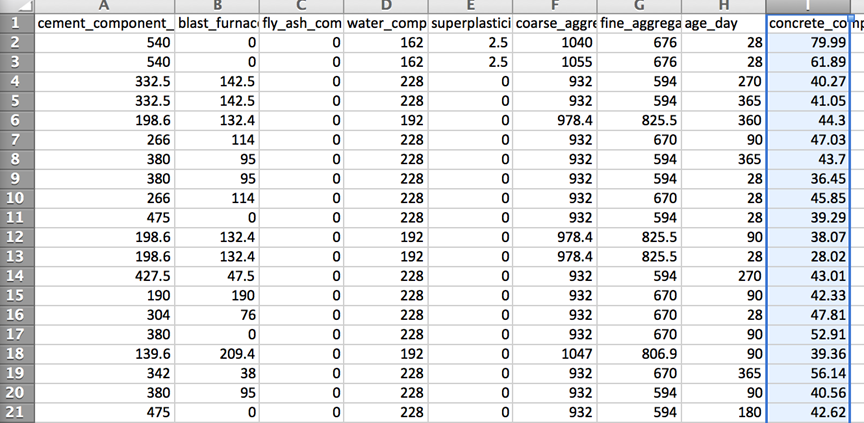
The example data tracks the concrete's compressive strength (MPa) compared to its cement, slag, fly ash, water, super plasticizer, coarse aggregate, and fine aggregate amounts (kg in a m3 mixture) and age (in days).

The dataset comes from the UC Irvine site: https://archive.ics.uci.edu/ml/machine-learning-databases/concrete/compressive/ and the exact version used for this case is concrete_data.csv (41KB). It contains 1030 observations. The first few rows are shown below:

Workflow

After importing this CSV data into Team Studio, the modeler can begin by analyzing the correlation between the compressive strength of concrete and the amount of cement used in the mixture.

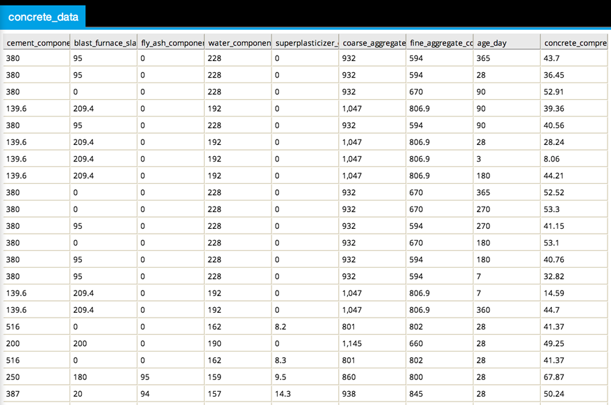
The modeler can create a new Data Flow with a DB Table element and then use the Preview option to view the data loaded within Team Studio, as shown below.

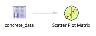
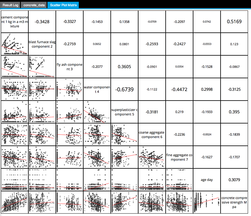
The data can be analyzed for linear dependencies using a Scatter Plot Matrix Operator with all columns selected, as follows:

Looking at a ScatterPlotGraph of the Concrete Strength related to the CementAmt reveals a general linear trend, scattered randomly around the trendline. As the amount of cement increases, there is a general overall increase in the strength of the concrete. This is a good indication that a linear regression analysis is worthwhile.

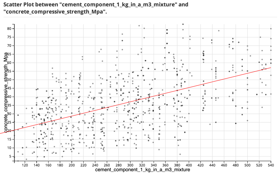
The modeler can then connect the Linear Regression Operator to the DB Table and perform an initial linear regression analysis using only the Concrete Strength(MPa) column as the suspected Dependent Variable and the Cement Amount column as the Independent Variable.

Results

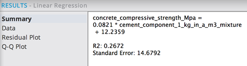
The results for this example show the following:

The Summary results tab shows an R2 of only 0.27, indicating that there are likely other factors than just the amount of cement in the mixture that affects the strength of the concrete. However, it does not necessarily mean that a linear model is not a good fit - the rest of the results should be analyzed.

The Data results tab displays:

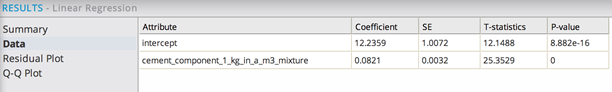
This linear regression analysis shows a very low p-value, well under the 0.05 threshold. This indicates a high level of confidence that the amount of cement in the mixture linearly affects the compressive strength of the concrete.

The strength of the linear relationship is represented by the Coefficient value of 0.0821. The bigger the Coefficient, the stronger the effect of Cement Amount on Concrete Strength. It represents the steepness of the Linear Regression line for forecasting Concrete Strength based on Cement column.

The Residual Plot displays the following graph:

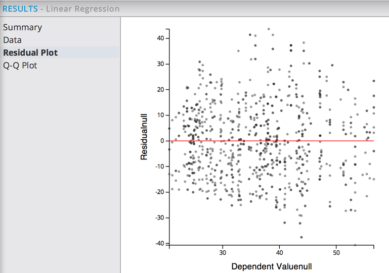
This shows a random pattern of Concrete Strength residuals around the Concrete Strength fit value horizontal line, suggesting that a Linear Regression model is a good fit for the data. There are no structure anomalies seen.

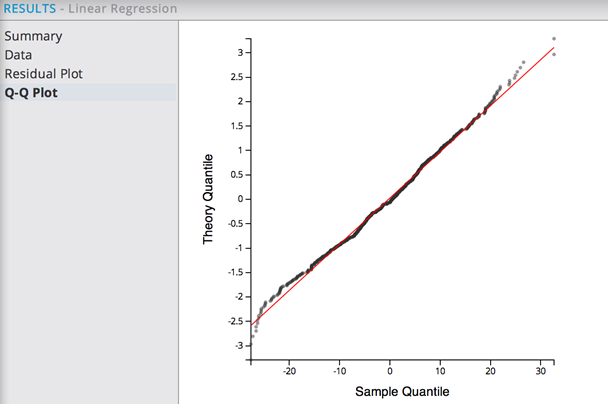
The Q-Q Plot shows the following graph:

This also indicates a good fit for there being a Linear relationship between CementAmt and Concrete Strength - that is, the prediction errors are normally distributed as expected.

Overall, the Linear Regression model seems like a good start, but because the R2 for the model is low when only analyzing one independent variable, the modeler might next want to try to add all of the available variables for the next linear regression analysis. The results for all of the variables being included in the regression show the following:

The Summary results tab shows the following information:

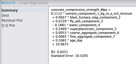
The R2, or accuracy of the model, has improved to 0.62 and the Standard Error has decreased.

The Data results tab shows the following table:

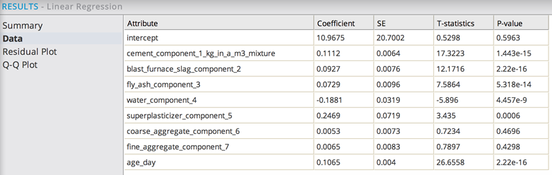
Sorting them by Coefficient value (clicking on the column header 'Coefficient') shows the Independent Variables, Superplasticizer, and Cement have the strongest linear correlation effect on the Concrete Strength.

Sorting them by P-value (clicking on the column header 'P-value') shows the Independent Variables, Age, Blast Furnace Slag, and Cement, have the highest confidence level in their significance in the model.

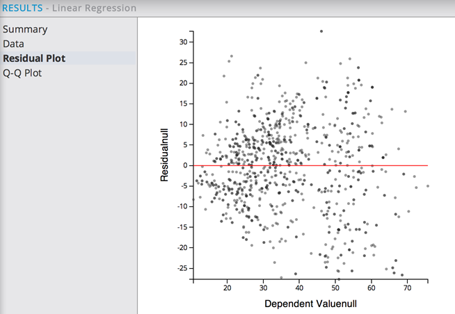
The Residual Plot again displays a random distribution of the Residuals around the Concrete Strength fit value horizontal line.

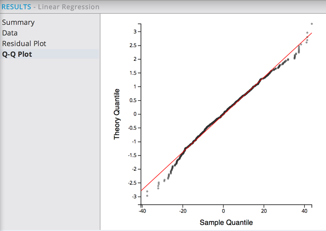
The Q-Q Plot again displays a normal distribution of the model's prediction errors.

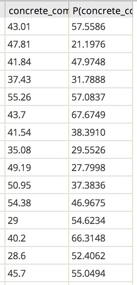
To obtain the Linear Regression model's predictions for the Concrete Strength based on the component amounts in the mixture, the modeler should add in the Linear Regression Prediction Operator and link it to both the DB Table source and the Linear Regression Operator, as follows:

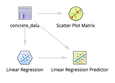
The results add an extra column to the data that provides the PredictedConcrete Strength value, P(MPa), in addition to the actual observed Concrete Strength value, MPa.

Summary

The lesson here is that although the obtained R2 is below the general 0.8 rule of thumb, an R2 of 0.62 is certainly an improvement over the initial model fit and the results overall still provide a nice linear regression model with all of the residual plots looking good.

Note: Either the un-modeled portion of the R2 is a factor orthogonal to the known data and, if found, could improve the model quality or it is just un-correlated noise and would not help enhance the model.

The modeler has to decide if the predictions provided by the model are "good enough" for the business goals at hand.