Logistic Regression Use Case (2)
Binomial logistic regression is used extensively in the medical and social sciences fields as well as in marketing applications that predict a customer's propensity to purchase a product.
Predicting Malignant Breast Cancer Cells based on Cell Measurements
From a UCI dataset dataset obtained from UCI website at: https://archive.ics.uci.edu/ml/machine-learning-databases/breast-cancer-wisconsin/ of patient cells with and without breast cancer, it was noticed that various characteristics and measurements of cells can provide significant modeling capabilities for predicting whether the cells are benign or malignant.
- Datasets
-
The exact dataset version used for this case is breast_cancer_data.csv (122KB).
It contains 569 observations, a diagnosis column, and 30 attributes related to cell nucleus properties (texture, perimeter, area, smoothness, compactness, concavity, concave points, symmetry and fractal dimension). The mean, standard error, and worst (largest) of these features were computed, resulting in 30 predictive features.
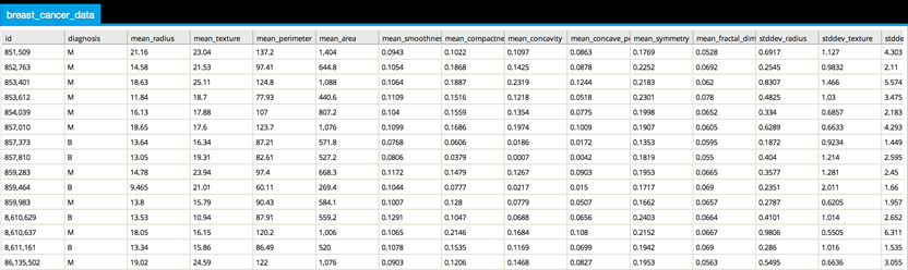
By loading the dataset into Team Studio, you can view the data using Data Explorer view (right-click the DB Table operator). The first few rows and columns are shown below:
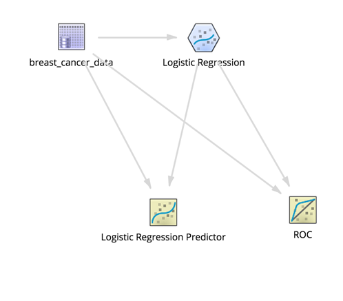
Workflow
The id is the patient ID and can be ignored. The diagnosis is the dependent variable to predict and can have a value of "M" for malignant or "B" for benign. The rest of the columns are numerical quantities obtained from a microscopic cell survey.
Because this model predicts a binary malignant or benign diagnosis, it makes sense to try the Logistic Regression operator.
Initially, the modeler might take the aggressive approach and select all the non-ID variables to be in the model.
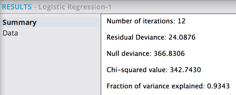
The Summary results tab shows:
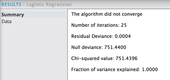
A number of bad diagnostic results are displayed.
The algorithm did not converge, as indicated by the Iteration amount being the maximum setting. The Residual deviance is essentially zero, which is suspicious because it makes the Chi square/ Null deviance indicate a near-perfect model fit (not likely).
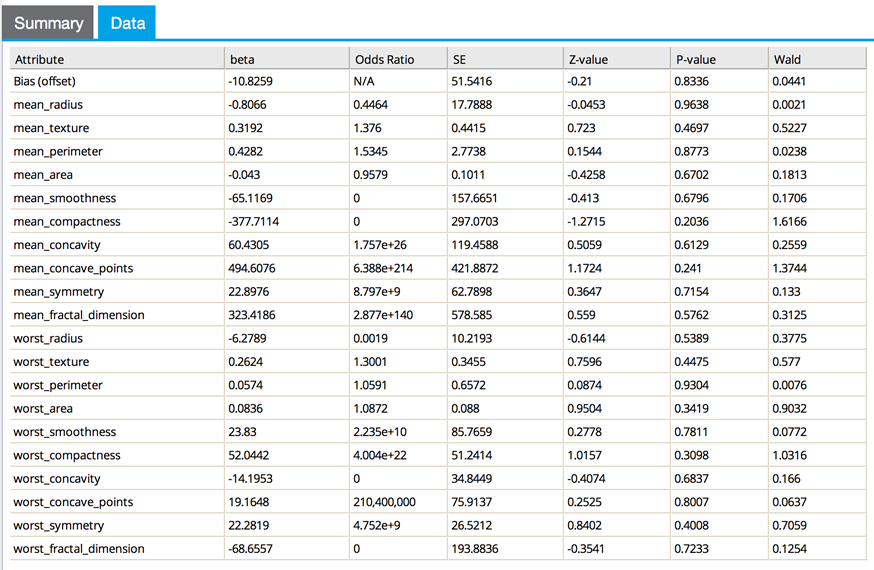
The Data results tab shows:
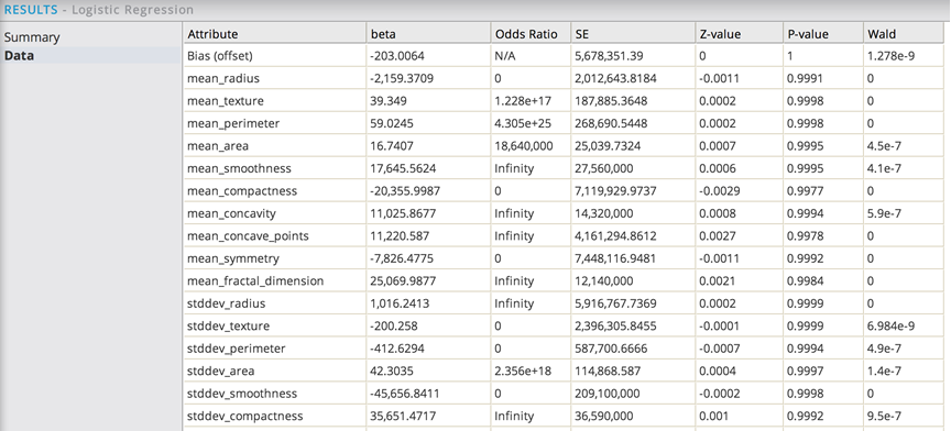
There are a number of large beta coefficient values, which is evidence the model was over fitting at least a subset of data. That would cause coefficients to run to infinity in logistic regression. In this case, the modeler would suspect all of the data is overfit because the model's deviance is zero. Overfitting means a very good fit on the training data that does not show the same utility on the new data.
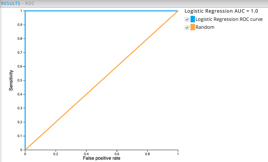
The ROC curve has a AUC of 1.0, which is definitely an indication of overfitting.
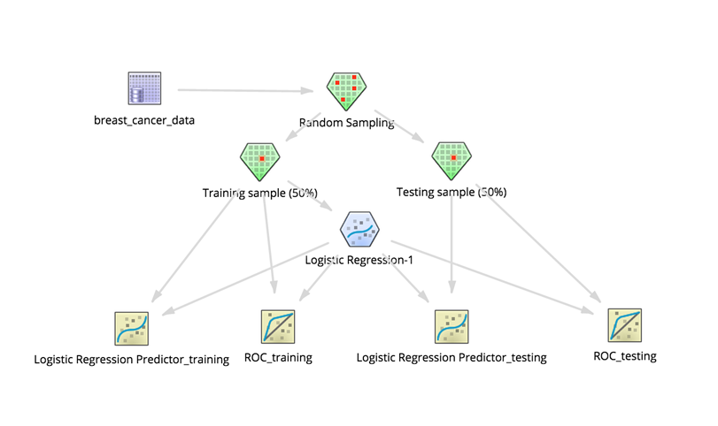
If the modeler suspects overfitting, a way to diagnose this is to run a cross-validation or "hold out" training where some data is restricted from the model and used to simulate new data. Inserting a Random Sampling operator to split the data into two 50% groups of sample data would accomplish this, as follows:
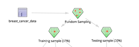
There should be two Sample Selector operators added to collect the split datasets.
Then adding two Logistic Regression Prediction operators to predict on the data used to build the model and on the non-training data allows the modeler to confirm whether the model only does well predicting using the training dataset.
Also adding ROC operators shows the quality of the model on both datasets. Note: the ROC operators hook up directly with the source dataset and the Logistic Regression operator.
The final cross-validation setup might look as follows:

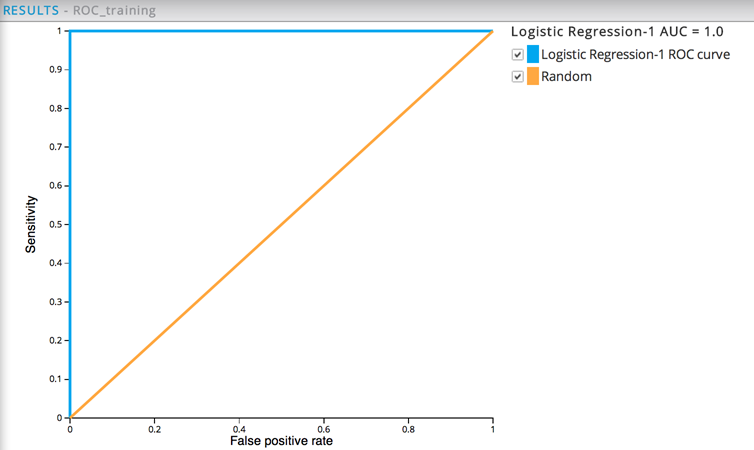
The resulting ROC graph for the training data shows a perfect model. The green not green in Illuminator line is always the diagonal and useless model. The red line shows the model performance. In the top right corner, it is 100% sensitive (that is, catches all the malignant cases) but has a high false positive rate (nearly always wrong). In the bottom left corner, it has zero false positives (never predicts malignant incorrectly) but has no sensitivity (no one is malignant). The top left corner shows pure model perfection with no false positives (everything predicted correctly) and complete sensitivity (everyone with malignancy was predicted).
The resulting ROC graph for the cross-validation data has the Area Under the Curve (AUC) of 0.9354 instead of 1. This is still excellent but is radically different than the training performance. For cross-validation purposes, the modeler wants the performance to be close - this much drop off is additional evidence of over fitting.

The ideal fix for over fitting in this case would be to obtain more training data in order to avoid the over-memorization of the data. However, the alternate, more realistic fix is to eliminate some of the variables, even though they might be useful in the model. With less training data, it is safer to have fewer training variables.
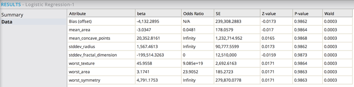
One approach for eliminating variables might be to turn on the stepwise regression methodology for the Logistic Regression operator, using stepwise mode using "AIC" criterion type.
In this example, the stepwise regression reduces the number of independent variables down to 7 from the original 30 variables. However, the model still has issues in this example with the odds ratio reaching Infinity for mean_concave_points, stddev_radius and worst_symmetry.
As another approach, the modeler might decide to manually remove the standard deviation columns in the data to begin with and rerun the regression without stepwise turned on. This might avoid using variables that duplicate each other's meanings. For example, the modeler might de-select the standard deviation columns from the model. This results in a converged model with reasonable p-values and no run-away coefficient values.
The Number of iteration times did not meet the maximum, which indicates the logistic regression converged appropriately.
The Data tab shows reasonable beta and Odds Ratio values.
The modeler can experiment iteratively by sorting the remaining variables by p-value and removing the ones with the highest p-values (that is, least confident of their significance). Note: the variables should not be taken out all at once because a variable may be bad because of another variable duplicating it. So it should be done in steps either manually or automatically, using stepwise.
This might leave the model down to just 3-4 variables, which is less likely to overfit. In the following example, only the variables mean.concavepoints, worst.area, mean.texture, and mean.radius have been left in the model. The results are:
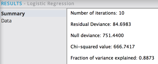
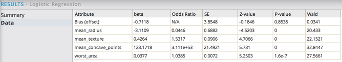
The p-values being very small give high confidence in their significance. Because the deviance of 84 is so low and the chi square/null deviance ratio is approximately .89, the modeler knows that just these 4 variables alone (mean.concavepoints, mean.texture, mean.radius, and worst.area) are predicting 89% of the diagnosis variation.
Because the p-values are within acceptable limits (under 0.05), then the modeler would sort by the coefficient values, looking for the variables with the strongest correlation effects.
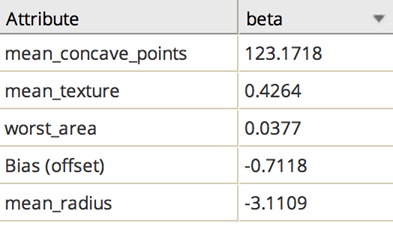
In this example, just looking at the mean.concavepoints variable's high coefficient value, the modeler knows it would be quite informative by itself if the model was run only with that independent variable. This model seems to be confirming the intuitive belief that the more non-round or abnormal cell shape/texture, the more chance of cancer.
Adding the ROC Graph operator helps analyze the quality of the model now. The AUC value of .9937 is very high but more believable than 1.0 earlier.
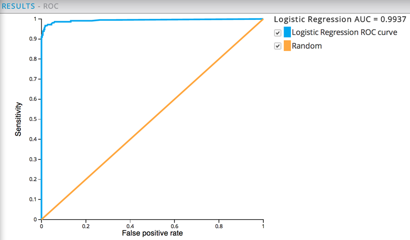
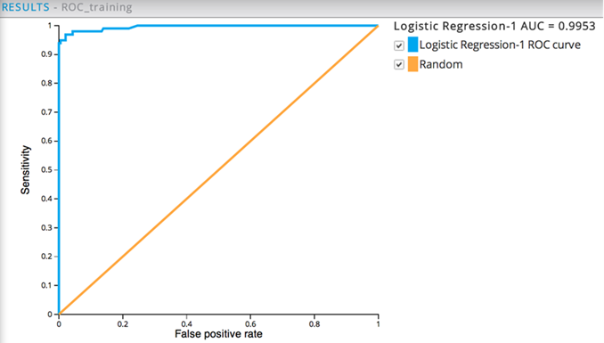
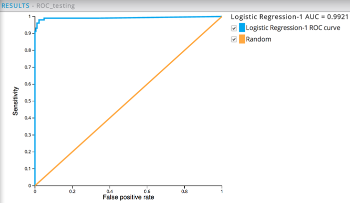
In this example, the two ROC graphs show nearly identical performance when the run against both the training dataset (AUC of .995) and non-training dataset (AUC of .992), which means the model is now a reliable predictor for cancer malignancy.
The modeler's hope is to find a simple model with fewer variables that shows good performance and that cross-validates and performs just as well on non-training data.
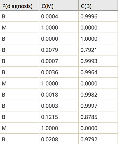
As a final step, the modeler would add the Logistic Regression Prediction operator for viewing the prediction column as well as the confidence level columns for both the training data and non-training data.
The prediction confidence levels are high for both the training data predictions and the non-training data predictions. The modeler can be confident in the quality of the logistic regression model. For example, in the first row shown below the predicted diagnosis is benign with more than 99% confidence in the prediction.