Generally, curve fit algorithms determine the best-fit parameters by minimizing a chosen merit function. In order to optimize the merit function, it is necessary to select a set of initial parameter estimates and then iteratively refine the merit parameters until the merit function does not change significantly between iterations. The Levenberg-Marquardt algorithm has been used for nonlinear least squares calculations in the current implementation.
The goodness of fit is shown as an R2-value. A value of R2=1.0 indicates a perfect fit, whereas R2=0.0 indicates that the regression model might be unsuitable for this type of data.
R2
The R2-value measures how much of the variation in the data points can be explained by the selected regression model:
![]()
![]()
where
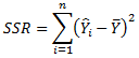 (the regression
sum of squares)
(the regression
sum of squares)
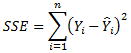 (the residual
or error sum of squares)
(the residual
or error sum of squares)
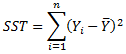 (the total sum
of squares, SST= SSE+SSR)
(the total sum
of squares, SST= SSE+SSR)
and ![]() represents
the ith fitted value (calculated
using the selected model) of the dependent variable Y.
represents
the ith fitted value (calculated
using the selected model) of the dependent variable Y.
Limitations to curve fitting
Since the calculation of the curve is an iterative process, the calculation must stop somewhere. In some cases, the maximum number of iterations might be reached before the best possible curve has been calculated. In that case, a message in the title bar of the visualization will inform you of this. In some cases, for example if the data is widely scattered or too few data points are available, the iterative process might also result in a curve that converges on a false minimum.
When a model is applied during data analysis, it is important not only to look at the R2-value and how well the curve fits the current markers in the scatter plot, but also to consider what the curve would look like for more extreme values and determine whether the model is reasonable in a scientific or statistical context. The number of unique x-values must be larger than, or equal to, the number of degrees of freedom in order to obtain a unique curve. If the curve can be solved in an infinite number of ways, it is not certain that the presented curve will be relevant to your data.
Heath, M.T., (2002), Scientific Computing: An Introductory Survey, 2nd ed., McGraw-Hill, New York.
Anderson, E., Bai, Z., Bischof, C., Blackford, S., Demmel, J., Dongarra, J., Du Croz, J., Greenbaum, A., Hammarling, S., McKenney, A., Sorensen, D., (1999), LAPACK Users' Guide, 3rd ed., Society for Industrial and Applied Mathematics, Philadelphia, PA, ISBN = 0-89871-447-8
References for Holt-Winters Forecast
Rob J Hyndman and George Athanasopoulos (2013), Forecasting: principles and practice. http://otests.com/fpp/7/1.
Rob J. Hyndman, Anne B Koehler, J. Keith Ord, and Ralph D. Snyder (2008), Forecasting with Exponential Smoothing: the state space approach, Springer.
See also: