Generalized Additive Models Example
This example is based on a data set described in Neter, Wasserman, and Kutner (1985, page 357; however, note that those authors fit a linear regression model to the data); it is also discussed in the documentation for the Nonlinear Estimation module, in the context of the Quick Logit Regression examples. In this example we will fit a generalized additive logit model to the data, which you can compare with the results computed for a ("simple") logit regression model. Detailed examples of generalized additive logit models and for other distributions and link functions are provided in Hastie and Tibshirani (1990).
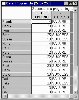
Suppose you want to study whether experience helps programmers complete complex programming tasks within a specified amount of time. Twenty-five programmers are selected with different degrees of experience (measured in months). They are then asked to complete a complex programming task within a certain amount of time. The binary dependent variable is the programmers' success or failure in completing the task. These data are recorded in the file Program.sta; shown below is a partial listing of this file.
- Specifying the Analysis
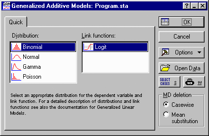
- Open the Program.sta data file. From the Data Mining menu, select Generalized Additive Models to display the Generalized Additive Models Startup Panel. Then select the Binomial distribution from the Distribution list; the Logit link function will automatically be selected.
Click OK, to display the GAM Specifications dialog, and click the Variables button to display a standard variable selection dialog. Select the variables for the analysis: Select Success as the dependent variable, and Expernce as the continuous predictor variable (in the third list of the 4-variable lists selection dialog). Click the OK button.
Note: STATISTICA automatically fills in the codes for the binomial dependent variable. During the computations, the value Failure in the dependent variable Success will be interpreted as 0, the value Success will be interpreted as 1. Hence, in the results, the greater the predicted (logit-) value, the greater is the probability of the programmers' success. - Reviewing Results
- Click OK on the GAM Specifications dialog to start the computations. A series of results spreadsheets and graphs will be produced.
As you can see, a number of results spreadsheets and graphs are reported to provide a comprehensive picture of the quality of the fit of the model and to aid in the interpretation of results. The interpretation of results from fitting generalized additive models is complex and requires experience (note that these techniques were only developed fairly recently, and there is not a large body of literature and "experience" with these techniques); Hastie and Tibshirani provide detailed discussions on how to interpret the results from these types of analyses, and more importantly, how to use this information to evaluate the appropriateness of the solutions obtained. You can also refer to Schimek (2000) for more recent developments regarding these techniques, and their applications.
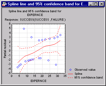
Let's only look at the result that is most characteristic for this method: The plot of the observed predictor values vs. the partial residuals (see also the GAM Introductory Overviews); this plot will also show the cubic spline fit for the final model.
To reiterate, this plot shows the final fitted cubic spline function, along with the observed predictor values, plotted against the partial residuals, i.e., against the residual values for the prediction of the (adjusted) dependent variable, after removing all other effects from the model (see Hastie & Tibshirani, 1990 for computational details; in particular formula 6.3 for the computation of adjusted dependent variable values). In this case, of course, there is only a single effect in the model. As you can see, the greater the experience of a programmer, the more likely is his or her success, as indicated by the monotone increasing cubic spline line.
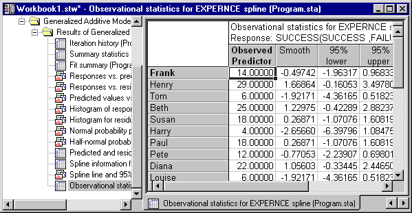
You can also review the various observational and residual statistics that are computed to identify outliers or any general lack of fit, or groups of cases that are not well represented ("explained") by the model.
- Fit Summary
- Now display the results spreadsheet labeled Fit summary. As briefly mentioned in the Introductory Overview, one of the important issues to consider when applying generalized additive models is whether the added smoothing - and the parameter that needs to be estimated to find the best cubic spline smoother - are "worth it," i.e., produce a significantly better fit of the model to the data. In this case, judging from the partial residual plot, the relationship between the predictor variables and the partial residuals appears almost linear.
Indeed, the Nonlinear p-value in the Fit summary spreadsheet is almost 1; thus, in this case is not clear whether the additional complexity of the additive logistic model is worthwhile.


