SANN Example 4: Time Series (Classification)

Data

IrisSNN.sta is a common data set used for classification purposes. The object is to assign 150 irises to one of three categories based on four measurements: sepal length and width, and petal length and width. The particular arrangement of this data set lends itself to time series classification data in that the frequency of switching between categories is low, and because of this, sequential values are likely to be from the same category. Part of the data set is shown in the following image.

This example explores some of the options that are available in Statistica Automated Neural Networks (SANN).

Click each process block to know the details.

Specifying the analysis

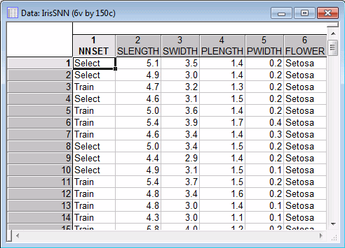
To begin the example, you can open IrisSNN.sta and start SANN in the following two ways:

• Ribbon bar. Select the Home tab. In the File group, click the Open arrow and select Open Examples to display the Open a Statistica Data File dialog box. Open the data file, which is located in the Datasets folder. Then, select the Statistics tab. In the Advanced/Multivariate group, click Neural Nets to display the SANN - New Analysis/Deployment Startup Panel. Or, select the Data Mining tab. In the Learning group, click Neural Networks to display the SANN - New Analysis/Deployment Startup Panel.
• Classic menus. From the File menu, select Open Examples. In the Open a Statistica Data File dialog, double-click the Datasets folder, and then double-click IrisSNN.sta. Then, from the Statistics menu or the Data Mining menu, select Automated Neural Networks to display the SANN - New Analysis/Deployment Startup Panel.

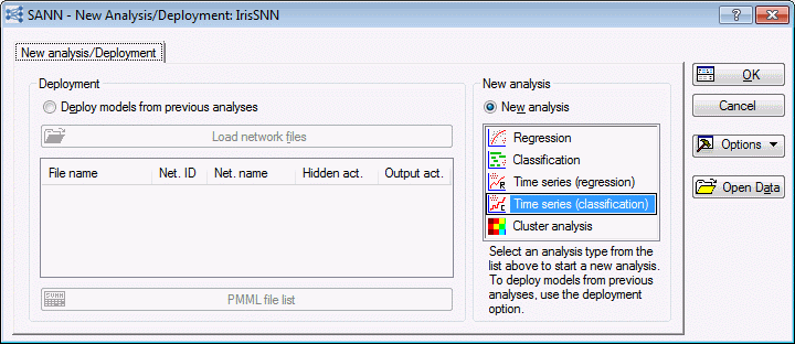
1. In the Startup Panel, you can select from five analysis types, or you can deploy previously saved networks. For this example, select Time series (classification) in the New analysis list.
   
2. Click the OK button to display the SANN - Data selection dialog box.
   
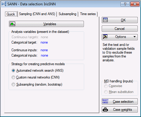
3. There are three types of strategies to choose from: the Automated network search (ANS), Custom neural networks (CNN), and Subsampling. For more details on the way to use ANS for time series analyses, see Example 3: Growth in Number of Airline Passengers over Time.
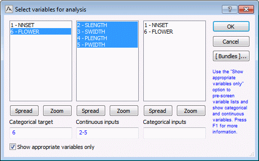
4. On the Quick tab of the SANN - Data selection dialog box, click the Variables button. In SANN, the types of variables you can select (example, categorical or continuous targets, categorical or continuous inputs) are pre-determined by your analysis selection. Because classification analysis presupposes a single categorical target with either continuous or categorical inputs, the variable selection dialog box does not provide an option for continuous targets.
5. For this example, first select the Show appropriate variables only check box. Then, select Flower as the Categorical target, and select Slength, Swidth, Plength, and Pwidth as Continuous inputs.
   
6. Click the OK button to return to the SANN - Data Selection dialog box.
   
7. In the Analysis variables (present in the dataset) group box, SANN reports that there are not any continuous targets.
8. In the Strategy for creating predictive models group box, select the Custom neural networks (CNN) option button.
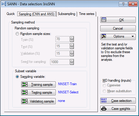
9. Select the Sampling (CNN and ANS) tab. As mentioned in Example 3, you are able to divide the data into two or three subsets (train, test, and validation) without disrupting the sequential nature of the data (see the Note on sampling in Example 3). For this example, we use a sampling variable to divide our data into two subsets: train and test.
10. Select the Sampling variable option button. The three buttons Training sample, Testing sample, and Validation sample are activated, enabling you to specify one or more of these samples.
    
11. Click the Training sample button to display the Sampling variable dialog box.
12. Click the Sample Identifier Variable button to display the Cross-Validation Specifications dialog box. For this example, select NNSET, and click the OK button.
13. In the Sampling variable dialog box, the Code for training sample field now defaults to Select. Change this field to Train (by double-clicking in the field to display a variable selection dialog box, selecting Train, and clicking OK).
14. In the Sampling variable dialog box, select the On option button in the Status group box.
    
15. Click the OK button, and repeat this process to specify the variable (NNSET) and code (Select) for the Testing sample. Once you have specified both subsets, the Data Selection dialog box - Sampling (CNN and ANS) tab should look as following image.
    
16. Select the Time Series tab, which contains options to set the values of the most important time series parameters, that is, Number of time steps used as inputs and Number of steps ahead to predict. For this example, we will leave these parameters at default, but depending on your future analyses, you might need to change these quantities so they reflect the time periodicity in your time series data. This is an additional decision that you need to make for time series problems – determining the number of time series steps to use as input to the network. For some problems, determining the correct number of input steps can require a certain amount of trial-and-error. However, if the problem contains a natural cycle period (such as the Series_G data set, which contains monthly sales figures, so there is a definite length - 12 - period in the data, see Example 3), you must try specifying that cycle, or an integral multiple of it.
17. In this case, we use the default values. By leaving the Number of steps used to predict set to 1, we can use a lag of 1 for making time series predictions.
18. Click the OK button in the SANN - Data Selection dialog box to display the SANN - Custom Neural Network dialog box.

Go back to the flow diagram.

Training the networks

The Custom Neural Network (CNN) tool enables you to choose individual network architectures and training algorithms to exact specifications. You can use CNN to train multiple neural network models with exactly the same design specifications but with different random initialization of weights. As a result, each network finds one of the possible solutions posed by neural networks of the same architecture and configurations. In other words, each resulting network provides you with a suboptimal solution (that is, a local minimum).

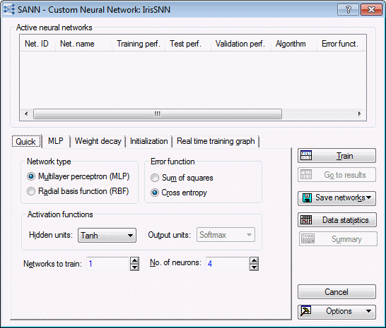
For this example, leave the number of Networks to train on the Quick tab at default. You can also experiment with the No. of neurons in the hidden layer. Usually there are no general guidelines to set this quantity, but if you want to make this process (that is, searching for the optimal value of neurons in the hidden layer) automated, then you can use the Automated Network Search (ANS).

Before we train our network, review some of the options available on the tabs of this dialog box. Look at the Quick tab.

Go back to the flow diagram.

Network type

SANN enables you to train either a multilayer perceptron (MLP) or a radial basis function (RBF) network. The multilayer perceptron is the most common form of network. It requires iterative training, the networks are quite compact and execute quickly once trained, and in most problems yield better results than the other types of networks including RBFs. In contrast, the radial basis function networks tend to be slower and larger than multilayer perceptron, and often have worse performance. They are also usually less effective than multilayer perceptrons if you have a large number of input variables (they are more sensitive to the inclusion of unnecessary inputs).

Go back to the flow diagram.

Error function

For classification analysis types, SANN enables you to select either Sum of squares error function or Cross entropy. By default, the cross entropy error function is used with Softmax as the output activation function. Such networks support a probabilistic interpretation of the output confidence levels generated by the network. They are true probability of input class memberships given the categorical levels of the target data.

Go back to the flow diagram.

Activation functions

SANN also provides options for specifying the activation functions for the input-hidden (hidden layer) and hidden-output (output layer) neurons of multilayer perceptron networks. You can always specify activation functions for the hidden units; however, you can only specify activation functions for the output units when the sum of squares error function is used. When the cross entropy function is used, Softmax is always used as the activation functions for output units.

1. For this example, we are using the defaults as shown before. Next, select the MLP tab.
   
2. On this tab, you can specify the training algorithm [Gradient descent, BFGS (Broyden-Fletcher-Goldfarb-Shanno), or Conjugate gradient] to use in training the multilayer perceptron (MLP) network, the Network randomization technique (you can initialize the network with values drawn from a Normal distribution or values from a Uniform distribution), and any Stopping conditions that you want to use.
3. You can use the defaults as shown. Next, select the Weight Decay tab.
   
4. You can use the options on this tab to specify the use of Weight decay regularization for the hidden layer, the output layer, or both. This option encourages the development of smaller weights, which tends to reduce the problem of over-fitting, thereby potentially improving generalization performance of the network.
5. Weight decay works by modifying the network error function to penalize large weights; the result is an error function that compromises between performance and weight size. Consequently, too large a weight decay term may damage network performance unacceptably, and experimentation is generally needed to determine an appropriate weight decay factor for a particular problem domain. For radial basis function (RBF) networks, you can only specify the use of weight decay for the hidden-output layer (output weight decay). For this example, do not use weight decay.

Go back to the flow diagram.

Reviewing the results

You have reviewed the various options in the SANN Custom Neural Network tool, click the Train button to train the neural networks. After training, the SANN - Results dialog box is displayed.

This dialog box contains six tabs and provides options for generating predictions and other results (example, confidences and accuracy), for performing graphical analysis of the data, for reviewing network statistics, for creating lift charts, for generating time series predictions, and for making custom predictions.

Reviewing the results

Perhaps the first result you should review is the list of retained networks, as well as their performance and specifications, which is displayed in the Active neural networks data grid displayed at the top of the Results dialog box. This information (also available in the Summary spreadsheet) enables you to quickly access the overall quality of your networks as well as their specific architectures and types, such as number of inputs, number of hidden units, activation types, etc.

For example, the network illustrated above in the Active neural networks grid and below in the Summary spreadsheet is type MLP with 4 inputs, 4 neurons in the hidden units, and 3 outputs (corresponding to the 3 categories of the target variable FLOWER), with a train and test classification rate at 96.5% and 97.10145%, respectively. The algorithm BFGS was used to train the network and the best solution was found at training cycle number 12. The network has a Tanh activation for the hidden units and Softmax activation function for the outputs (and hence the use of the Entropy error function).

Just because the classification rate of a network is high, it does not mean the solution found by the network is a good one. For example, a network trained on a data set with an unbalanced target variable consisting of 90% of category, say, A, and 10% of category B is likely to predict most of the 90% of the patterns belonging to A while unable to correctly predict cases belonging to B. Such a network can yield a high classification rate but also an output that is almost flat.

Given the above, you need to examine the performance of your networks with more depth rather than just considering the performance rates. One way to do this is to examine the confusion matrix and the percentage of correctly classified cases per category. You can print this information in a spreadsheet by clicking the Confusion matrix button on the Details tab of the Results dialog. The confusion matrix and classification summary are useful tools in evaluating the effectiveness of a classification network. To review these two spreadsheets, click the Confusion matrix button. Both spreadsheets are generated.

The confusion matrix shows both the number of correctly classified cases per category as well as the number of incorrectly classified cases per category. For example, from the above spreadsheet we note that the network has correctly classified all 27 cases of category Setosa in the train set. Also 25 cases out of a total of 26 belonging to Versicol are correctly classified, leaving us with the remaining 1 misclassified case, in favor of Setosa. Similar analysis can be carried out for the Virginic class, which has 26 cases out of a total of 27 correctly classified, with 1 misclassified case.

The above information is further summarized in the classification summary spreadsheet, where we can see the percentage of classified cases for Setosa, Versicol, and Virginic. Note that the network is consistent in its classification rate, that is, it classifies all categories with similar classification rates.

Equally important for a classification analysis is the study of lift charts and the ROC (Receiver Operator Characteristic) curves. For more details, see the step-by-step example The Iris Problem.

Finally, after completing your analysis and approving the network you have trained, the last step is to save the network so you can use it later. This process, that is, using a network for predicting future data, is known as deployment. With Statistica, you can deploy SANN PMML models using either the Rapid Deployment module or SANN itself, but first you must save your networks.

Go back to the flow diagram.