Example 6: Hypotheses About the Noncentrality Parameter of the F Distribution
There are many potential uses for the Noncentral F Probability Calculator. In Examples 4 and 5, we demonstrate some classic applications - computing power for the traditional F-tests in ANOVA. Here, we discuss a very simple technique that proves useful in some of our later exercises. This technique is to test a hypothesis about the noncentrality parameter δ of a noncentral F distribution, on the basis of a single observation from that distribution.
Since the noncentrality parameter is related directly to other interesting quantities, we can use this technique to test hypotheses about these quantities. For example, in Example 9 we show how to use this technique to test hypotheses of "minimal fit" in the analysis of variance.
The technique is extremely simple. Suppose we have an observation from an F distribution with ν1 and ν2 degrees of freedom. Consider some "minimal value of interest" a for the noncentrality parameter. We want to test the null hypothesis H0: δ <= c against the alternative hypothesis H1: δ > c.
The general technique is as follows:
- Choose a Type I error rate, α.
- Find the 1 - α cumulative probability point in the noncentral F distribution with ν1 and ν2 degrees of freedom, and noncentrality parameter equal to c. Call this value F*.
- If the observed F statistic exceeds F*, reject the null hypothesis in favor of the alternative.
As a concrete example, suppose you had an F statistic with 3 and 36 degrees of freedom, and wanted to test the null hypothesis that the noncentrality parameter is less than or equal to 2, with α = .01. To find the critical value for this one-tailed hypothesis test, perform the following steps.
Ribbon bar. Select the Statistics tab. In the Advanced/Multivariate group, click Power Analysis to display the Power Analysis and Interval Estimation Startup Panel.
Classic menus. From the Statistics menu, select Power Analysis to display the Power Analysis and Interval Estimation Startup Panel.
In the Startup Panel, select Probability Distributions and Noncentral F Distribution.
Click the OK button to display the Noncentral F Probability Calculator.
Select the (1 - Cumulative p) check box.
In the Numerator df box, enter 3.
In the Denom. df box, enter 36.
In the Delta box, enter 2, the noncentrality parameter.
In the 1 - Cum. p box, enter .01.
In the Compute group box, select the F option button so that Statistica will compute the value of F at the requested percentage point.
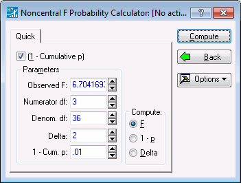
Click the Compute button. The result should look like the image below.
The critical value is approximately 6.704. Besides computing the critical value, you can compute the probability level for any observed value of F. Suppose, while performing this test, you obtain an observed value of 7.35. What is the probability level of this value?
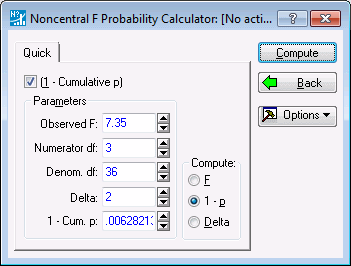
Simply enter 7.35 in the Observed F box, and select 1 - p as the quantity to Compute. Click the Compute button, and the calculator should appear as below.
The probability (.00628) is, of course, less than .01, since the value is higher than the critical value at the .01 level that we just established.
In Example 9, we show how to test nonstandard tests of minimal effect in the analysis of variance, using the technique from this example.
See also, Power Analysis - Index.


