Example 6: Factor Analysis with an Intercept Variable

The data file for the example is Boll310.sta.

In this example, 5 judges were asked to estimate, to the nearest tenth of an inch, the length of lines drawn on 60 index cards, with one line per card.  

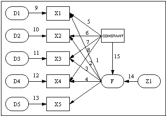
Judge 1 gave his estimates to the nearest tenth of a centimeter, while the other four judges gave their ratings to the nearest tenth of an inch. The rating process is modeled with a single factor model. The ratings of each judge are modeled as arising through multiplicative (representing a rater-specific variance) and additive (representing rater-specific mean) transformations of the true length, represented by the factor F. So, for example, the ratings that we see for rater X1 are the true length, multiplied by a factor loading, with a rater-specific constant added on.

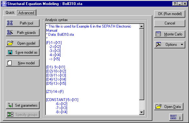
The PATH1 commands for this model are in the file Boll310.cmd.

The primary purpose for using the factor model in this case is to gauge differences among the raters. Indeed, the scale for the underlying latent variable is arbitrary. We fix the scale by setting the factor loading for rater 5 to be fixed at 1.0, and the additive constant for rater 5 to be fixed at zero.

The path diagram for the model is shown below.

The manifest variable CONSTANT is actually an artificial manifest variable with a mean of 1 and a variance of zero. It contributes no variance, and adds a constant to variables that load on it.

To analyze this example using an intercept variable, you must select the Moments option button under Data to analyze on the Analysis Parameters dialog (accessed by clicking the Set parameters button on the Structural Equation Modeling Startup Panel, Advanced tab.

In that case, the augmented moment matrix is analyzed, and the artificial variable CONSTANT is added automatically to the list of available manifest variables.