Statistica Gage Linearity Technical Notes

Measurement systems are not perfect, and the accuracy of their readouts is limited by various sources of error that cannot be controlled. These sources of error may stem from the nature of the gage itself, or they might be related to the conditions under which a gage operates. Some of these errors are deterministic and some are random in nature. Either way, such sources of error result in imperfections in gage readouts that need to be taken into account in many industrial applications of Process Analysis.

Measurement errors can be quantified using the so called accuracy and precision. Accuracy measures the difference between readings of the gage and the true value of the quantity that has been measured. This is in contrast to precision, which measures variations in a gage's readings over repeated measurements relative to a sample of reference values. Note that measurements may suffer from one or both sources of error.

As mentioned above, due to various uncontrollable factors, the accuracy of an instrument may vary according to the operating conditions under which measurements are made. One of those operating conditions is the range (magnitude or size) of the quantity of measurement. For instance, one might use an ometer to determine the electrical resistance of various conductors. Similarly, one might use a nanometer to measure the dimension of objects of different thickness. None of these instruments are capable of yielding measurements with the same accuracy across the entire measurement range.

The accuracy associated with the measurements of a gage can be broken down into three main components: linearity, bias, and stability. Linearity provides us with an estimate of how accurate a measurement process is over an expected range (which is naturally taken to be the operating range of the gage). In other words, it answers the question "how does my gage accuracy vary as the measurement range changes?" or "how does the measurement range affect the accuracy of my gage?"

The second component, bias, measures how different your gage measurements are from a set of reference values (i.e., a set of values that are taken to be reliable and accurate) at one particular location (i.e., value of the measurement variable).

Thus, while the bias measures the difference between the readings of a gage with those of a reference sample at a specific location, linearity measures the change in that difference (i.e., bias) over a certain range (which for practical reasons is chosen to be the normal operating range of the gage).

The third component, stability, provides us with the answer to "how does accuracy change over time," thus providing guidance as to how often a gage may require calibration (see AIAG - Automotive Industry Action Group manual).

Gage Linearity and Bias

To determine the linearity and bias of a gage (a measuring device), select a minimum of g 5 parts. By lay out inspection, measure the reference values for each selected part and make sure that the operating range of the gage is encompassed. Then measure each part a number of m times, where m 10. Against each reference value (x-axis) plot the individual biases and their average value (y-axis), and perform a line fit, i.e., find the slope and intercept (constant) of a line, i.e., bias = intercept + slope x reference, which best describes the relationship between the reference values and the bias using the least-squares method. Denoting the individual reference values as x_i and the average biases as y_i the slope and intercept of this line is estimated from:

where n is the number of measurements, x_i is the ith reference value and y_i is the ith value of the bias. Note that once we obtain an estimate of the slope and intercept, we are able to predict the value of the bias y_o for an arbitrary reference point x_o.

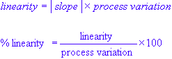
The linearity is measured as the absolute value of the regression slope multiplied by the estimate of the process variation. Thus:

where denotes the absolute value. The bias is given by the difference between the actual measurement outcome and the respective reference value. Equally, the percentage of bias is given by the percentage of the overall process variation:

In order for a gage linearity to be acceptable, the line defined by zero bias, i.e., bias = 0, must fall entirely within the region of the graph defined by the lower and upper bounds of the confidence intervals of the fitted line.

Regression Diagnostics

After constructing a regression model often it is necessary to verify how well the model fits the data and, hence, its ability to accurately predict future observations. This section provides the necessary diagnostic tools for verifying the regression process. For further details see Statistica Multiple Regression.

Regression Statistics

SSError. Sum of squares error due to unexplained variability in the data

SSRegression. Sum of squares error due to the regression

SSTotal. Total sum of squares error

R². Often called the coefficient of determination. It is defined as the ratio of the sum of squares explained by the regression model and the total sum of squares

The R²can also be expressed in terms of the SS_Error

Thus the more the regression fits the data the closer R² is to unity.

Multiple R

Known as the coefficient of multiple correlation, which is the positive square root of R-square (the coefficient of multiple determination, see Computational Approach - Residual Variance and R-square). This statistic is useful in multivariate regression (i.e., multiple independent variables) when you want to describe the relationship between the variables.

Values of R² close to 1 indicate a small difference between the observations and the predicted values made by the regression model. The quantity R² x 100 yields the percentage of variation accounted for by the least-squares method. See Computational Approach - Residual Variance and R-square for further details.

R² (adjusted). Derived from theR² weighted by the number of variables and observations according to the formula:

where n is the number of observations and p is the number of predictor variables. Thus the R² (adjusted) measures the goodness of fit while taking account the number of predictors in the model.

Standard error

Measures the error on the prediction of a regression. In other words the standard error measures the dispersion of the observed values about the regression line:

Regression Table

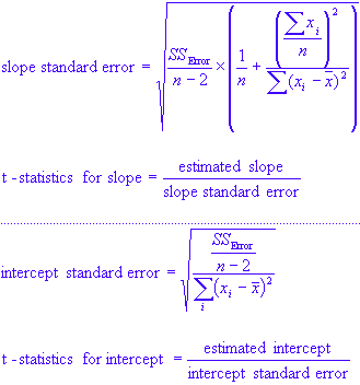
A linear regression problem is uniquely determined by the estimated values of its parameters, i.e., the slope and the intercept (constant). However, since these parameters are often calculated from noisy data sets of finite size, there is always a finite but non-zero uncertainty associated with their estimates. These uncertainties are measured using the standard error and its associated t-statistics. The standard error for the slope of linear model and its intercept (constant) are given by:

It should be noted that the uncertainty in estimates of the parameters of the regression model approaches zero as the number of observations increases (see Qazaz).

ANOVA Table

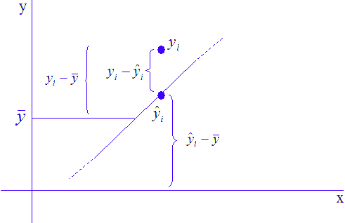
As stated before, the total sum of squares SS_Total of a regression problem is the sum of the regression and error sum of squares, i.e., SS_Regression + SS_Error. SS_Regression is the variation explained by the regression, while SS_Error represents the unexplained component of the variance due to noise on the dependent variable. The total variation in the regression problem is, therefore, given by:

Total variation = SS_Regression + SS_Error

In a sense, error sum of squares S_Error is a manifestation of the uncertainty in the regression problem due to the existence of noise (imperfections) in the dependent variable. Alternately, regression sum of squares SS_Regression is an estimate of the uncertainty in the regression model due to the finite nature of the dataset.

Divided by the number of degrees of freedom, the total sum of squares SS_Total provides an estimate of variability in the regression problem. For the regression component, the degrees of freedom is given by the number of predictors, while for the error component it is given by n - 2, where n is the number of observations. Consequently, the total number of degrees of freedom for the regression problem is n - 1, which is the sum of the number of degrees of freedom for both components of variation.

The variance explained by the regression is the regression sum of squares divided by the number of degrees of freedom. It is also known as the mean square error MSE:

Similarly, the unexplained variance due to noise is given by:

Given the above, the total variance is then derived from:

The null hypothesis that all source of variability comes from the regression is then given by:

Note: F and the resulting p-value are used as an overall F-test of the relationship between the dependent variable and the set of predictors.

Bias Significance Table

The bias of each measurement, i.e., the difference between each measurement and the reference value, is given by:

Using the above we can then calculate the average bias for the ith part using:

where m is the number of measurements per part. The p-values are calculated to test whether the bias is zero at each reference point. STATISTICA Gage Linearity provides you with two distinct methods for calculating the standard deviation. The first method is based on the sample range:

where d₂ is taken from statistical tables (see Duncan for more details). Note that when more than one part has the same master (reference) value the estimate of the standard deviation is based on:

The second method is based on the sample measure of the standard deviation:

You can use any of the above to calculate the standard deviation, which in turn is used to calculate the t-statistics:

The p-value is then calculated as the probability of T<t for the two tailed t-distribution with degrees of freedom equal to that of the error variance.

See also, Example 5: Gage Linearity and Bias Study.

Copyright © 2021. Cloud Software Group, Inc. All Rights Reserved.