Example 8: Testing for Circumplex Structure
The data matrix, from Guttman (1954), is in the Guttman.sta data file.
This data file, used frequently to demonstrate a Guttman circumplex, is a correlation matrix among 6 different kinds of abilities for 710 Chicago school children.

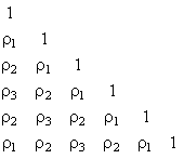
A perfect circumplex correlation matrix (Guttman, 1954) has equal correlations on sub-diagonal strips. For example, a 6x6 correlation matrix would be of the form:
A circumplex hypothesis is an example of a correlational pattern hypothesis. (See Steiger, 1980a for a review of the literature on pattern hypothesis testing.) A pattern hypothesis is any hypothesis that specifies correlations are equal to each other, or to specified numerical values. SEPATH can perform any pattern hypothesis on 1 or more correlation matrices.
A circumplex hypothesis is a pattern hypothesis within a single population. Frequently, comparisons of correlations across populations are of interest as well as comparisons within populations. SEPATH can test pattern hypotheses across samples as well as within samples.
The general approach to testing correlational pattern hypotheses with SEPATH is straightforward.
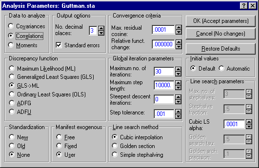
(1) Select the Correlations option button under Data to analyze on the Analysis Parameters dialog.
(2) Click the Path tool button on the Structural Equation Modeling Startup Panel, Quick tab or Advanced tab, to display the Path Construction Tool dialog, where you create all the paths for a correlation matrix for the relevant variables. Select the Correl. option button under Path Type, then highlight all of the manifest variables you want to test in the To: column.
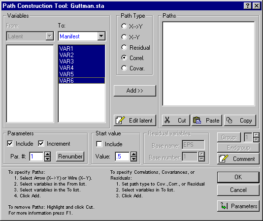
(3) Click the Add>> button to creates all the paths for the full correlation matrix for the manifest variables.
(4) Click the OK button to save the model.
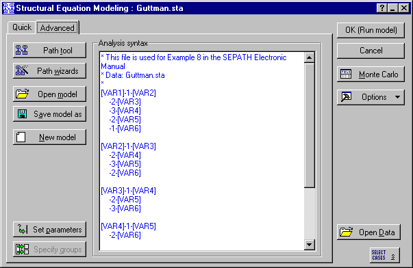
(5) Edit the model to apply the required constraints.
The commands for testing a hypothesis of circumplex structure are in the file Circle.cmd.
Test these commands. Select the Correlations option button under Data to analyze on the Analysis Parameters dialog.
The sample size is very large in this example. Hence, we would expect the precision of estimation to be very high. At the same time, we would have to keep in mind that the "reject-support" approach of the Chi-square test would be of very limited usefulness in this situation. We recognize that a model with as many constraints as this one will almost certainly not fit perfectly in the population, and we have very high power to detect an imperfect fit.
The Chi-square statistic yields, in this case, a value of 27.05 with 12 degrees of freedom. The probability level is .008, indicating that the null hypothesis of perfect fit must be rejected. Jöreskog (1978), analyzing these data, remarked that they "do not fit a circumplex well."
This conclusion seems, in the 20-20 vision of hindsight, unjustified, and incorrect. A more reasonable conclusion is that it is highly probable that they do not fit a circumplex perfectly. Goodness-of-fit indices indicate how well these data actually do fit a circumplex. The 90% confidence interval for the Steiger-Lind (1980) RMS index is between .021 and .064.
The corresponding confidence interval for the adjusted population gamma coefficient is between .972 and .997.
A reasonable conclusion would seem to be that Guttman's data fit a circumplex very well, a fact that we have verified statistically.