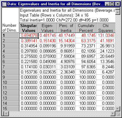
Example 2.1: Analyzing an Indicator Matrix (Consumer Preferences)
This example is based on a data set presented by Hoffman and Franke (1986). The purpose of this example is to present a brief illustration of a typical application of correspondence analysis in marketing research. For an introductory example demonstrating the basic principles of correspondence analysis (including the role of supplementary points), see Example 1. Refer also to the Introductory Overview for a general discussion of correspondence analysis, and the interpretation of typical results.
The example data file Beverage.sta contains data for a group of male and female MBA students from Columbia University who were asked to indicate the frequency with which they purchased and consumed various soft drinks in a 1-month period. The data for the 34 subjects were coded into a binary indicator matrix: a 1 was entered for the respective beverage if the respective subject indicated purchase and consumption at least every other week, and a 0 was entered if the respective subject indicated purchase or consumption less than every other week. For each of the 8 popular soft drinks used in this study, a second variable was created that was coded as the inverse of the respective first variable, that is, a 1 was entered if the respective beverage had not been consumed or purchased, and a 0 if it had been consumed or purchased over the previous month. Shown following is a partial listing of the data coded in this manner for 8 popular soft drinks. Open the Beverage.sta data file using the menu; it is in the Statistica/Examples/Datasets directory.
This manner of coding might seem unusual at first; however, indicator matrices are discussed in the Introductory Overview - MCA. In particular, the standard correspondence analysis of an indicator matrix gives the same results as a multiple correspondence analysis of the data tabulated in the more standard form (example, where there is only one variable Coke, with two codes Yes and No, see example data file Beverag2.sta). This is demonstrated briefly in Example 2.2.
This example explains typical application of correspondence analysis in marketing research.

Specifying the analysis
- Select Correspondence Analysis from the Statistics - Multivariate Exploratory Techniques menu to display the Correspondence Analysis (CA): Table Specifications Startup Panel.
- On the Correspondence Analysis (CA) tab select the Frequencies w/out grouping vars option button under Input.
- Select the variables. Click the Variables with frequencies button to display the standard variable selection dialog box.
- Select all variables and then click the OK button.
- Click the OK button on the Startup Panel to perform the correspondence analysis. After a few moments the Correspondence Analysis Results dialog box is displayed.
Reviewing the results
Reviewing and interpreting the coordinates
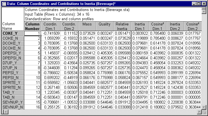
- Click the Row and column coordinates button on the Advanced tab. The spreadsheet with the column coordinates contains the following values.
- It appears that all beverages are reasonably well represented by the two-dimensional solution, only Diet Pepsi has a Quality value of less than .5.
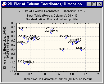
- Now plot the beverages in the two-dimensional space. On the Advanced tab, click the Column, 2D button.
- A careful review of the graph suggests that the first axis mostly distinguishes between diet beverages and non-diet beverages, while the second dimension appears to separate the colas from the non-colas.
Plotting the row-coordinates
You could now also plot the row coordinates, that is, the individual subjects who participated in the study, in the two-dimensional coordinate system. This enables you to distinguish ("graphically") between different segments of consumers, that is, those who do or do not drink diet beverages, and who do or do not drink colas. Moreover, if you carefully review the statistics for the row coordinates you can see that the largest contributors to the inertia for the second dimension are cases number 13 and 28. These points almost solely define the direction of the second dimension.


